clustering k-Means gaussian-mixture-models GNBC EM-algorithm scikit-learn digits machine-learning unsupervised-learning python ipynb Expectation-Maximization Algorithm For Gaussian Mixture Models
Objectives
In this article we will
- train a Gaussian NBC with the EM algorithm
- compare the results you get to those of the k-Means clustering provided in Scikit-learn
Background and Tools
The EM (Expectation-Maximisation) algorithm solves the problem of not being able to compute the Maximum Likelihood Estimates for unknown classes directly by iterating over the two steps until there is no significant change in Step 2 observable:
-
Compute the expected outcome for each sample / sample given estimates for priors and distribution (essentially, the likelihoods for observing the sample assuming an estimated distribution)
-
Compute the new estimates for your priors and distributions (in the case of a Gaussian NBC, new means and variances are needed) based on the estimated expected values for how much each sample belongs to the respective distribution.
You can find the algorithm stated explicitly as given in Murphy, “Machine Learning - A probabilistic perspective”, pp. 352-353 HERE.
One special case of the EM algorithm is k-Means clustering, for which an implementation can be found in Scikit-learn.
Implementation task
1. Implement the EM-algorithm to find a Gaussian NBC for the digits dataset from Scikit-learn (you can of course also use the MNIST_Light set from Lab 5, but for initial tests the digits data set is more convienent, since it is smaller in various aspects). You may assume (conditional) indepdendence between the attributes, i.e., the covariances can be assumed to be simply the variances over each attribute. Split the data set in 70% training, 30% test data. If you experience problems due to the repreated multiplication of tiny values in likelihoods, it might help to normalise the data to values between 0.0 and 1.0 (i.e., simply divdie every pixel value with 16.0 in the digits data).
Collecting the dataset
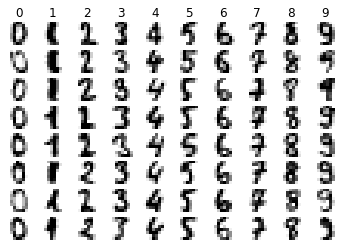
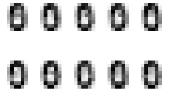
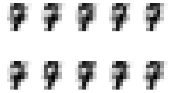
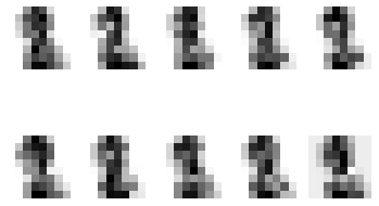
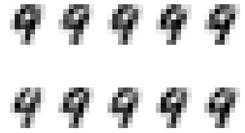
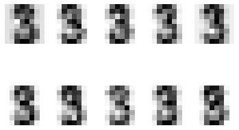
Recall that the digits dataset consists of 1,797 samples. Each sample is an 8x8 image of a single handwritten digit from 0 to 9. Each sample therefore has 64 features, where each of the 64 features is a brightness value of a pixel in the image.
from sklearn.datasets import load_digits
digits = load_digits()
print('Shape of digits.images input array:', digits.images.shape)
Shape of digits.images input array: (1797, 8, 8)
digits.data
array([[ 0.,  0.,  5., ...,  0.,  0.,  0.],
       [ 0.,  0.,  0., ..., 10.,  0.,  0.],
       [ 0.,  0.,  0., ..., 16.,  9.,  0.],
       ...,
       [ 0.,  0.,  1., ...,  6.,  0.,  0.],
       [ 0.,  0.,  2., ..., 12.,  0.,  0.],
       [ 0.,  0., 10., ..., 12.,  1.,  0.]])
Visualising the data
import matplotlib.pyplot as plt
import numpy as np
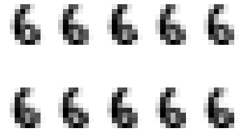
# Display random sample of images per class
n_samples = 8
n_classes = 10
for cls in range(n_classes):
    idxs = np.where(digits.target == cls)[0]
    idxs = np.random.choice(idxs, n_samples, replace=False)
    for i, idx in enumerate(idxs):
        plt.subplot(n_samples, n_classes, i * n_classes + cls + 1)
        plt.axis('off')
        plt.imshow(digits.images[idx], cmap=plt.cm.gray_r, interpolation='nearest')
        if i == 0:
            plt.title(str(cls))
plt.show()
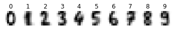
# Display mean image of each class
cls_means = np.zeros(shape=(10,8,8))
for cls in range(n_classes):
    idxs = np.where(digits.target == cls)[0]
    cls_means[cls] = np.mean(digits.images[idxs], axis=0)
    plt.subplot(1, n_classes, cls + 1)
    plt.axis('off')
    plt.imshow(cls_means[cls], cmap=plt.cm.gray_r, interpolation='nearest')
    plt.title(str(cls))
plt.show()
Splitting into training and test sets
num_examples = len(digits.data)
print('Total examples:', num_examples)
Total examples: 1797
split = int(0.7*num_examples)
print('Training set examples:', split)
Training set examples: 1257
train_features = digits.data[:split]
train_labels = digits.target[:split]
test_features = digits.data[split:]
test_labels = digits.target[split:]
print("Shape of train_features:", train_features.shape)
print("Shape of train_labels:", test_labels.shape)
Shape of train_features: (1257, 64)
Shape of train_labels: (540,)
print("Number of training examples:", len(train_features))
print("Number of test examples:    ", len(test_features))
print("Number of total examples:   ", len(train_features)+len(test_features))
Number of training examples: 1257
Number of test examples:     540
Number of total examples:    1797
Normalising the data
train_features = train_features / 16.0
test_features = test_features / 16.0
Implementing the EM-algorithm
The pseudocode for this algorithm has been provided by the EDAN95, Ht2 2019 teaching staff. The full algorithm can be found in “Machine Learning - A Probabilistic Approach”, Murphy (pp. 353-354).
  EM-for-GMM(X, K)
    1. Initialise theta_(0,k) = (pi_(0,k), mu_(0,k), sigma_(0,k))
      pi_k is the class prior for class k (e.g. assume uniform distribution here initially)
      mu_k are the means for the attribute values j in class k (e.g., the means over a random subset of the data)
      sigma_k is the covariance for the attribute values in class k (can be simplified to a variance lower_sigma_(jk, 2) for each attribute j if a G-NBC is assumed as the model)
    2. Iterate over E and M steps as follows:

3. Stop, when the mu_k and sigma_k are not changing signficantly anymore.
EM-algorithm with a Gaussian NBC assumption
import pandas as pd
from scipy.stats import multivariate_normal, mode, norm
class EMforGMM:
def __init__(self, K, tol, epsilon, max_iter):
self.K = K
self.tol = tol
self.epsilon = epsilon
self.max_iter = max_iter
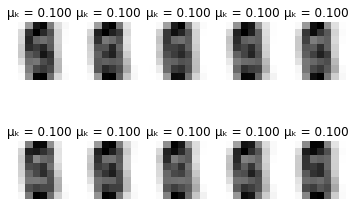
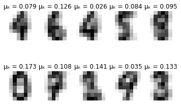
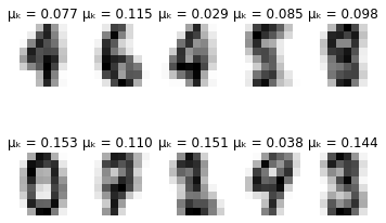
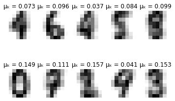
def plot_updates(self, means, covs, weights):
fig = plt.figure()
for k in range(self.K):
plt.subplot(2, 5, k + 1)
plt.axis('off')
plt.imshow(np.reshape(means[k], (8,8)), cmap=plt.cm.gray_r)
plt.title(f'\u03BC\u2096 = {weights[k]:.3f}')
plt.show()
def compute_prob(self, X, mu, sigma):
return 1/np.sqrt(2*np.pi*sigma) * np.exp(-1/(2*sigma) * (X - mu)**2)
def fit(self, X):
n_samples, n_features = np.shape(X)
# Priors
pi = np.full(shape=self.K, fill_value=(1/self.K))
# Means
mu = np.ones(shape=(self.K, n_features))
# Covariances
sigma = np.ones(shape=(self.K, n_features))
# Initialisation
idxs = np.resize(range(self.K), n_samples)
np.random.seed(42)
np.random.shuffle(idxs)
for k in range(self.K):
mu[k] = np.mean(X[idxs == k], axis=0)
sigma[k] = np.var(X[idxs == k], axis=0)
sigma += self.epsilon
delta_mu = np.inf
delta_sigma = np.inf
P = np.zeros(shape=(n_samples, self.K))
r = np.zeros(shape=(n_samples, self.K))
pi_k = np.zeros(self.K)
for i in range(self.max_iter):
# Plot learned representation every 10 iterations
if i % 10 == 0:
print('-'*8 + ' iteration %i ' % i + '-'*8)
print(u'\u0394\u03BC\u2096:', delta_mu)
print(u'\u0394\u03C3\u2096:', delta_sigma)
self.plot_updates(mu, sigma, pi)
# 1. E-step: compute likelihood
for k in range(self.K):
P[:, k] = np.prod(self.compute_prob(X, mu[k], sigma[k]), axis=1)
r = pi * P / (np.sum(pi * P, axis=1)).reshape(-1,1)
# 2. M-step: update means and variances
r_k = np.sum(r, axis=0)
pi_k = pi
pi = r_k / np.sum(r_k)
for k in range(self.K):
mu_k = np.sum(r[:, k].reshape(-1,1) * X, axis=0) / r_k[k]
delta_mu = np.abs(mu[k] - mu_k).max()
mu[k] = mu_k
sigma_k = np.diag((r[:, k].reshape(-1,1) * (X - mu[k])).T @ (X - mu[k]) / r_k[k]) + self.epsilon
delta_sigma = np.abs(sigma[k] - sigma_k).max()
sigma[k] = sigma_k
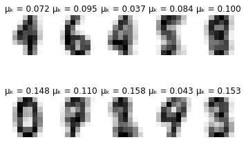
# Convergence condition
if np.linalg.norm(pi_k - pi) < self.tol:
print('-'*8 + ' converged' + '-'*8)
self.plot_updates(mu, sigma, pi)
break
self.weights_ = pi
self.means_ = mu
self.covariances_ = sigma
Training the model
Parameters
K: Number of clusters (Gaussians) to form.tol: Absolute error criterion (convergence threshold) between successive iterations. EM iterations will stop once this lower bound condition has been satisfied.epsilon: Scalar smoothing value added to the covariances (sigma).max_iter: Mximum number of training iterations to perform (terminates early if convergence threshold is reached).
K = 10
tol = 1e-10
epsilon = 1e-4
max_iter = 160
model = EMforGMM(K, tol, epsilon, max_iter)
model.fit(train_features)
-------- iteration 0 --------
Δμₖ: inf
Δσₖ: inf
-------- iteration 10 --------
Δμₖ: 0.02042206092031973
Δσₖ: 0.006980384032168101
-------- iteration 20 --------
Δμₖ: 0.0043815616448701356
Δσₖ: 0.0011309086525828627
-------- iteration 30 --------
Δμₖ: 0.0017659929216632952
Δσₖ: 0.0007651120346653245
-------- iteration 40 --------
Δμₖ: 0.00015692821124366207
Δσₖ: 0.00010460936069779658

-------- iteration 50 --------
Δμₖ: 4.857764125190678e-05
Δσₖ: 3.239725424089568e-05

-------- iteration 60 --------
Δμₖ: 6.6351084939964e-06
Δσₖ: 4.4816080131682146e-06

-------- iteration 70 --------
Δμₖ: 5.103103453807378e-06
Δσₖ: 1.4159123793711093e-06

-------- iteration 80 --------
Δμₖ: 2.3776945110021153e-07
Δσₖ: 1.6398608126966252e-07

-------- iteration 90 --------
Δμₖ: 3.2171004027414796e-08
Δσₖ: 2.183106893871578e-08
-------- iteration 100 --------
Δμₖ: 5.7718268497986e-09
Δσₖ: 3.933698297653443e-09

-------- iteration 110 --------
Δμₖ: 1.1219926099315103e-09
Δσₖ: 7.656876105377464e-10

-------- converged--------

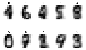
Visualising the model results
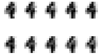
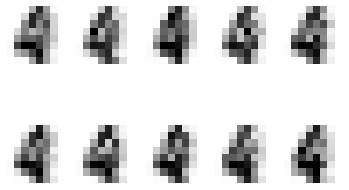
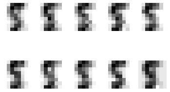
# Generating digits using learnt distributions
for i in range(10):
    for j in range(10):
        pixels = np.array([np.random.normal(model.means_[i][pixel], model.covariances_[i][pixel]) for pixel in range(64)])
        plt.subplot(2, 5, j + 1)
        plt.axis('off')
        plt.imshow(pixels.reshape((8,8)), cmap=plt.cm.gray_r, interpolation='nearest')
    plt.show()
Clustering training data
2. Use the results of the EM-algorithm (the found distribution parameters) to cluster the training data (esentially, using the resulting classifier to do a prediction over the training data). Produce a confusion matrix over the known labels for the training data and your EM-generated clusters. What do you see?
class GNB:
    def __init__(self, gmm):
        self.gmm = gmm

    def fit(self, K):
        self.K = K
        self.means = self.gmm.means_
        self.covs = self.gmm.covariances_
        self.weights = np.log(self.gmm.weights_)

    def predict_single(self, x):
        f = lambda i: self.weights[i] + multivariate_normal.logpdf(x, mean=self.means[i], cov=self.covs[i])
        return np.argmax(
            np.fromfunction(np.vectorize(f), shape=(self.K,), dtype=int)
        )

    def predict(self, X, translate_targets=True):
        y_pred = np.apply_along_axis(self.predict_single, axis=1, arr=X)
        return y_pred
gnb = GNB(model)
gnb.fit(K)
y_pred = gnb.predict(train_features)
from sklearn import metrics
from mlxtend.plotting import plot_confusion_matrix
print('-'*10 + 'Classification Report' + '-'*5)
print(metrics.classification_report(train_labels, y_pred))
print('-'*10 + 'Confusion Matrix' + '-'*10)
plot_confusion_matrix(metrics.confusion_matrix(train_labels, y_pred))
----------Classification Report-----
              precision    recall  f1-score   support

           0       0.00      0.00      0.00       125
           1       0.00      0.00      0.00       129
           2       0.20      0.07      0.11       124
           3       0.01      0.01      0.01       130
           4       0.01      0.01      0.01       124
           5       0.06      0.09      0.07       126
           6       0.00      0.00      0.00       127
           7       0.00      0.00      0.00       125
           8       0.00      0.00      0.00       122
           9       0.19      0.30      0.23       125

    accuracy                           0.05      1257
   macro avg       0.05      0.05      0.04      1257
weighted avg       0.05      0.05      0.04      1257

----------Confusion Matrix----------
print("Accuracy: %s" %(metrics.accuracy_score(train_labels, y_pred)))
print("Completeness score: %s" %(metrics.completeness_score(train_labels, y_pred)))
print("Homogeneity score: %s" %(metrics.homogeneity_score(train_labels, y_pred)))
print("AMI score: %s" %(metrics.adjusted_mutual_info_score(train_labels, y_pred)))
Accuracy: 0.046937151949085126
Completeness score: 0.5536596800547269
Homogeneity score: 0.5320086662948669
AMI score: 0.5358345474756068
Repairing cluster assignments
3. If necessary, find a way to “repair” the cluster assignments so that you can do a prediction run over the test data, from which you can compare the results with your earlier implementation of the Gaussian NBC.
Method 1. Reassign class labels manually
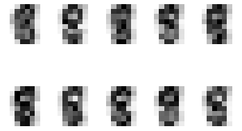
# Visualise cluster assignments
fig = plt.figure()
for k in range(K):
    img = np.reshape(gnb.means[k], (8,8))
    plt.subplot(2, 5, k + 1)
    plt.axis('off')
    plt.imshow(img, cmap=plt.cm.gray_r, interpolation='nearest')
    plt.title(str(k))
plt.show()
# "Repair" training set predictions
y_train = np.zeros(len(y_pred))
y_train[y_pred == 0] = 1
y_train[y_pred == 1] = 6
y_train[y_pred == 2] = 4
y_train[y_pred == 3] = 5
y_train[y_pred == 4] = 8
y_train[y_pred == 5] = 0
y_train[y_pred == 6] = 7
y_train[y_pred == 7] = 2
y_train[y_pred == 8] = 9
y_train[y_pred == 9] = 3
print('Repaired training set cluster assignments...')
print('-'*10 + 'Classification Report' + '-'*5)
print(metrics.classification_report(train_labels, y_train))
print('-'*10 + 'Confusion Matrix' + '-'*10)
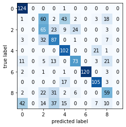
plot_confusion_matrix(metrics.confusion_matrix(train_labels, y_train))
Repaired training set cluster assignments...
----------Classification Report-----
              precision    recall  f1-score   support

           0       0.67      0.99      0.80       125
           1       0.41      0.29      0.34       129
           2       0.33      0.52      0.40       124
           3       0.45      0.67      0.54       130
           4       0.61      0.23      0.33       124
           5       0.69      0.58      0.63       126
           6       1.00      0.94      0.97       127
           7       0.76      0.84      0.80       125
           8       0.47      0.48      0.48       122
           9       0.28      0.12      0.17       125

    accuracy                           0.57      1257
   macro avg       0.57      0.57      0.55      1257
weighted avg       0.57      0.57      0.55      1257


    ----------Confusion Matrix----------
The downside to this approach is that we have to manually alter the assigned class labels for both the train and test set predictions.
Method 2. Create target mapping function
class GNB:
    def __init__(self, gmm):
        self.gmm = gmm

    def fit(self, K, X_train, y_train):
        self.K = K
        self.means = self.gmm.means_
        self.covs = self.gmm.covariances_
        self.weights = np.log(self.gmm.weights_)

        self.create_target_mapping(X_train, y_train)

    def create_target_mapping(self, X_train, y_train):
        self.target_mapping = np.zeros(self.K)
        y_pred = self.predict(X_train, translate_targets=False)
        for i in range(self.K):
            indexes = y_pred == i
            self.target_mapping[i] = mode(y_train[indexes])[0][0]

    def predict_single(self, x):
        f = lambda i: self.weights[i] + multivariate_normal.logpdf(x, mean=self.means[i], cov=self.covs[i])
        return np.argmax(
            np.fromfunction(np.vectorize(f), shape=(self.K,), dtype=int)
        )

    def predict(self, X_test, translate_targets=True):
        y = np.apply_along_axis(self.predict_single, axis=1, arr=X_test)
        return self.target_mapping[y] if translate_targets else y
# Prediction run over training data
gnb = GNB(model)
gnb.fit(K, train_features, train_labels)
y_pred = gnb.predict(train_features, translate_targets=True)
print('Prediction over training data...')
print('-'*10 + 'Classification Report' + '-'*5)
print(metrics.classification_report(train_labels, y_pred))
print('-'*10 + 'Confusion Matrix' + '-'*10)
plot_confusion_matrix(metrics.confusion_matrix(train_labels, y_pred))
Prediction over training data
----------Classification Report-----
              precision    recall  f1-score   support

           0       0.67      0.99      0.80       125
           1       0.00      0.00      0.00       129
           2       0.33      0.52      0.40       124
           3       0.45      0.67      0.54       130
           4       0.54      0.82      0.65       124
           5       0.69      0.58      0.63       126
           6       1.00      0.94      0.97       127
           7       0.76      0.84      0.80       125
           8       0.47      0.48      0.48       122
           9       0.00      0.00      0.00       125

    accuracy                           0.58      1257
   macro avg       0.49      0.59      0.53      1257
weighted avg       0.49      0.58      0.53      1257

----------Confusion Matrix----------
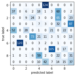
# Prediction run over test data
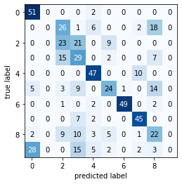
y_pred = gnb.predict(test_features, translate_targets=True)
print('Prediction over test data...')
print('-'*10 + 'Classification Report' + '-'*5)
print(metrics.classification_report(test_labels, y_pred))
print('-'*10 + 'Confusion Matrix' + '-'*10)
plot_confusion_matrix(metrics.confusion_matrix(test_labels, y_pred))
Prediction over test data
----------Classification Report-----
              precision    recall  f1-score   support

           0       0.59      0.96      0.73        53
           1       0.00      0.00      0.00        53
           2       0.30      0.43      0.35        53
           3       0.32      0.55      0.40        53
           4       0.70      0.82      0.76        57
           5       0.57      0.43      0.49        56
           6       0.98      0.91      0.94        54
           7       0.75      0.83      0.79        54
           8       0.33      0.42      0.37        52
           9       0.00      0.00      0.00        55

    accuracy                           0.54       540
   macro avg       0.45      0.54      0.48       540
weighted avg       0.46      0.54      0.49       540

----------Confusion Matrix----------
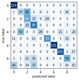
Compare to k-Means with Scikit-learn
4. Use now also the k-Means implementation from Scikit-learn and compare the results to yours (they should be similar at least in the sense that there are classes that are more clearly separated from the rest than others for best approaches).
from sklearn.cluster import KMeans
clf = KMeans(n_clusters=len(np.unique(train_labels)), init='random')
clf.fit(train_features, train_labels)
KMeans(init='random', n_clusters=10)
# Compute the clusters
y_pred = clf.fit_predict(test_features)
“Because k-means knows nothing about the identity of the cluster, the 0-9 labels may be permuted. We can fix this by matching each learned cluster label with the true labels found in them” – J. VanderPlas, 2016.
# Permute the labels
labels = np.zeros_like(y_pred)
for i in range(10):
    mask = (y_pred == i)
    labels[mask] = mode(test_labels[mask])[0]
mat = metrics.confusion_matrix(test_labels, labels)
print('-'*10 + 'Classification Report' + '-'*5)
print(metrics.classification_report(test_labels, labels))
print('-'*10 + 'Confusion Matrix' + '-'*10)
plot_confusion_matrix(metrics.confusion_matrix(test_labels, labels))
----------Classification Report-----
              precision    recall  f1-score   support

           0       0.98      0.96      0.97        53
           1       0.55      1.00      0.71        53
           2       1.00      0.74      0.85        53
           3       0.00      0.00      0.00        53
           4       0.98      0.93      0.95        57
           5       0.91      0.95      0.93        56
           6       0.95      1.00      0.97        54
           7       0.69      1.00      0.82        54
           8       0.00      0.00      0.00        52
           9       0.43      0.82      0.56        55

    accuracy                           0.74       540
   macro avg       0.65      0.74      0.68       540
weighted avg       0.65      0.74      0.68       540

----------Confusion Matrix----------
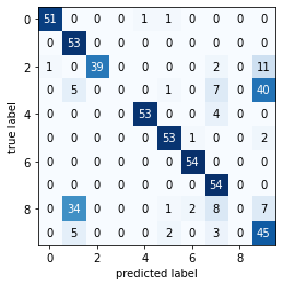
print("Accuracy: %s" %(metrics.accuracy_score(test_labels, labels)))
print("Completeness score: %s" %(metrics.completeness_score(test_labels, labels)))
print("Homogeneity score: %s" %(metrics.homogeneity_score(test_labels, labels)))
print("AMI score: %s" %(metrics.adjusted_mutual_info_score(test_labels, labels)))
Accuracy: 0.7444444444444445
Completeness score: 0.8089661544736777
Homogeneity score: 0.7128614631464921
AMI score: 0.7508813410219344
Credits
This assignment and its instructions were prepared by EDAN95 course coordinator E.A. Topp, link here.
Label permutation problem for k-Means clustering of digits dataset explained in detail here.
2019-12-13 00:00:00 -0800 - Written by Jonathan Logan Moran