decision-trees CART ID3 supervised-learning classification machine-learning numpy scikit-learn digits python ipynb Decision Trees for Multinomial Classification
Introduction
What is covered in this post:
- Scikit-learn’s
DecisionTreeClassifer(based on CART) - Scikit-learn’s
GridSearchCV - Classification with the Scikit-learn
digitsdataset - ID3 algorithm from scratch
Often times, classification can be framed as a sort of questioning-answering system. Questions are asked about the input data which aid the model in determining a prediction. One example of a “question” that a model might ask is does this input image contain this attribute value? Decision trees naturally help to structure this kind of if-then hierarchical decision-making by defining a series of questions that lead to a class label or value. In this article, we will explore several algorithms for constructing the two types of decision trees: the ID3 algorithm for Classification Trees and CART analysis for Regression Trees. We’ll start with the CART Regression Tree implementation from Scikit-learn and eventually work our way to the ID3 algorithm. While reading along, you will be able to implement your own ID3 algorithm from scratch using the code provided in this notebook. Let’s get started…
1. Built in Scikit-learn DecisionTreeClassifier
Objective #1: Use and experiment with the built-in Scikit-learn DecisionTreeClassifier (based on CART)
Scikit-learn digits dataset
1. Load the digits dataset from the datasets provided in Scikit-learn. Inspect the data. What is in there?
For this classification task, we will be using the Scikit-learn digits dataset. Recall that the digits dataset consists of 1797 samples across 10 classes. Each sample is an 8x8 image of a single handwritten digit from 0 to 9. Each sample therefore has 64 features, where each of the 64 features is a brightness value of a pixel in the image.
from sklearn.datasets import load_digits
digits = load_digits()
Now that we’ve got our data loaded, let’s take a look at a sample of the images in the dataset.
digits.data
array([[ 0.,  0.,  5., ...,  0.,  0.,  0.],
       [ 0.,  0.,  0., ..., 10.,  0.,  0.],
       [ 0.,  0.,  0., ..., 16.,  9.,  0.],
       ...,
       [ 0.,  0.,  1., ...,  6.,  0.,  0.],
       [ 0.,  0.,  2., ..., 12.,  0.,  0.],
       [ 0.,  0., 10., ..., 12.,  1.,  0.]])
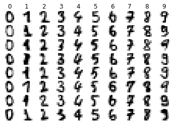
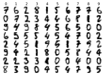
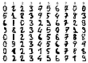
We can see from the above that each pixel is stored in an array. The pixel value is represented by an integer between 0 and 16. To get a better look at the data visually, we can run the following code to preview a few samples of each class chosen at random.
import numpy as np
import matplotlib.pyplot as plt
def visualize_random(images, labels, examples_per_class=8):
    """
    Display a sample of randomly selected images per class
    """
    number_of_classes = len(np.unique(labels))

    for cls in range(number_of_classes):
        idxs = np.where(labels == cls)[0]
        idxs = np.random.choice(idxs, examples_per_class, replace=False)
        for i, idx in enumerate(idxs):
            plt.subplot(examples_per_class, number_of_classes, i * number_of_classes + cls + 1)
            plt.imshow(images[idx].astype('uint8'), cmap=plt.cm.gray_r, interpolation='nearest')
            plt.axis('off')
            if i == 0:
                plt.title(str(cls))
    plt.show()
visualize_random(digits.images, digits.target, examples_per_class=8)
2. Split your data set into 70% training data (features and labels), and 30% test data.
from sklearn.model_selection import train_test_split
X_train, X_test, y_train, y_test = train_test_split(digits.data, digits.target, test_size=0.3)
print("Number of training examples: ",len(X_train))
print("Number of test examples: ",len(X_test))
print("Number of total examples:", len(digits.data))
Number of training examples:  1257
Number of test examples:  540
Number of total examples: 1797
NOTE: We would typically rescale the images’ pixel values prior to running the data through our model. In the case of the digits data, the pixel values are in the range [0-16]. In order to rescale the images, we would divide the pixel values by a factor equal to the maximum pixel value (16.0). This would transform every pixel value from the range [0-16] to [0,1].
Rescaling, in general cases, is important for two main reasons:
- Maintaining consistency across datasets whose images have differing pixel ranges, and
- Preserving the learning rate across the data.
Without scaling, images with higher pixel ranges contribute more to the loss than those with lower ranges. The learning rate cannot update effectively to compensate for this if the images have different or high ranges.
Now, with that out of the way–we will not be scaling the digits data for use with the ID3-algorithm. Decision trees are said to be invariant to feature scaling, and in the case of the ID3-algorithm, scaling the image data to continuous values could actually result in overfitting (many more branch points at each split). Continuous attribute values like scaled pixel intensities can also be more time-consuming to process with the ID3-algorithm (source: Wikipedia).
Scikit-learn DecisionTreeClassifier
3. Set up a DecisionTreeClassifier as it comes in Scikit-learn. Use it with default parameters to train a decision tree classifier for the digits dataset based on the training data. Follow the tutorial (or the respective documentation) and produce a plot of the tree with graphviz if you have it available. What can you learn from this about how the used algorithm handles the data?
As mentioned earlier, Scikit-learn’s DecisionTreeClassifier is based on the CART (Classification and Regression Tree) algorithm. Like the name suggests, CART can produce either Classification or Regression trees depending on whether the dependent variable (the target or class variable) is categorical or continuous, respectively. Both the ID3 and CART algorithm are greedy algorithms, meaning that they both choose the “best” feature locally that splits the data with the greatest discriminative power. In statistic and machine learning, a discriminator is a model that divides a set of classes or categories of items. So, the term discriminative power refers to how effective a discriminator is at categorising or dividing items correctly.
What is different about the CART and ID3 algorithms, however, are the functions used to calculate discriminative power. Referred to as the splitting criterion, the CART algorithm uses Gini impurity as a measure of non-homogeneity, whereas the ID3 algorithm uses information gain as its splitting criterion. While the difference between these two formulas will not be discussed in this notebook, you may choose to read more about them in-detail here.
from sklearn import tree
# Initialising with default parameters
classifier = tree.DecisionTreeClassifier()
The DecisionTreeClassifier is capable of performing multinomial (multi-class) classification on a dataset. We will initialise the decision tree learner with its default parameters for now, then attempt to optimise it by tweaking the criterion, max_depth, min_samples_split and min_samples_leaf. If you want to get a head start on what these parameters are, check out the official scikit-learn documentation here.
# Fitting the decision tree on training set
sklearnDigitsTree = classifier.fit(X_train, y_train)
Calling the fit() method on our digits training data will build a corresponding decision tree model. Without getting into the specifics of the exact implementation, our decision tree algorithm will run as follows:
- Select the best attribute which splits the data.
- Make that attribute a decision node and break the data into subsets.
- Recursively build branches for each child until one of the stopping crtieria are met:
- There are no remaining samples to split, or
- There are no remaining attributes to split on (all samples are of the same class).
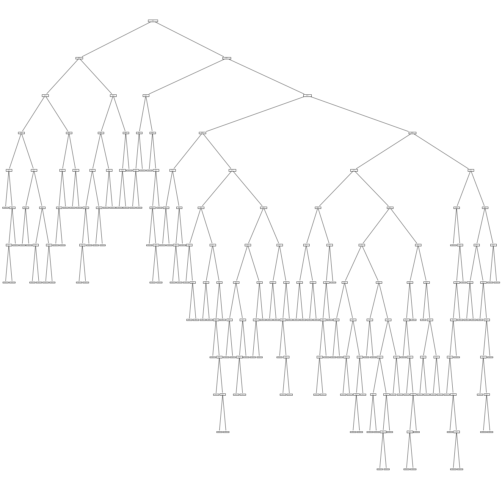
# Visualising the tree using scikit-learn
from sklearn.tree import plot_tree, export_text
The following bit of code lets us display the resulting decision tree within our Jupyter notebook.
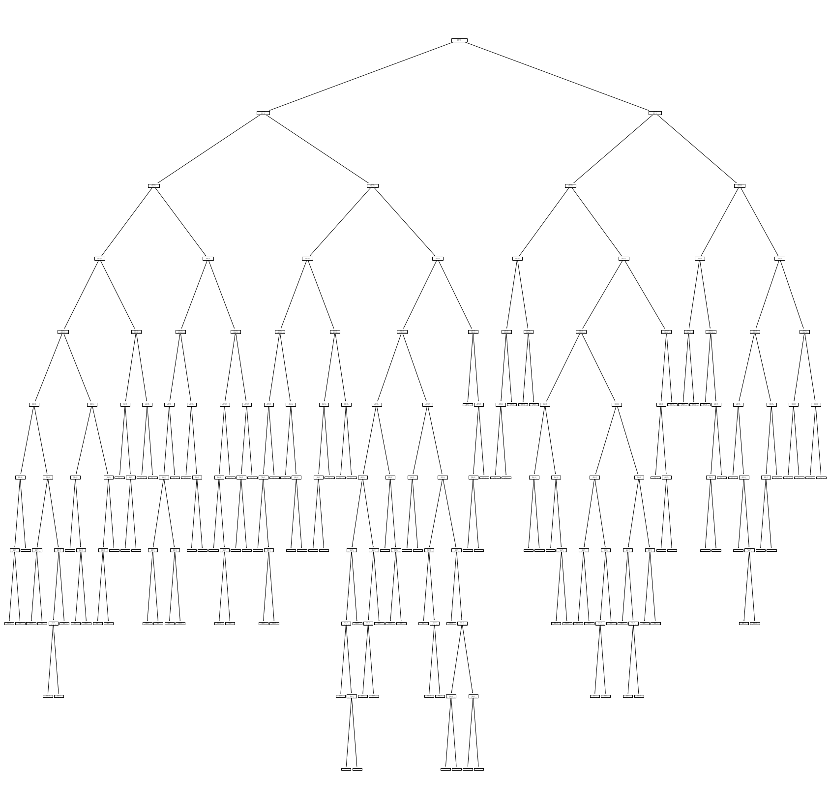
plt.figure(figsize=(20,20))
tree.plot_tree(sklearnDigitsTree)
plt.show()
There are other ways to visualise a decision tree, one of which involves the use of the Python graphviz library. Since we are writing our own model in the later part of the notebook, we will install the requirement here (now is also a good time to make sure that the pydot dependency is installed).
# Visualising the tree using graphviz
!pip install graphviz
Requirement already satisfied: graphviz in /usr/local/lib/python3.7/dist-packages (0.10.1)
4. Test the classifier with the remaining test data and analyse it using the metrics packages of Scikit-learn (classification_report, confusion_matrix). What do you see?
Now, we will perform a prediction run over the test data using the decision tree that we previously fit. In essence, the test samples will be classified by sorting them down the tree from the root to a leaf/terminal node where a class label is provided. Each node in the tree acts as a test case for some attribute (i.e. an “if” statement), and each edge descending from the node corresponds to the possible answers to the test case (KDnuggets, 2020).
y_pred = classifier.predict(X_test)
from sklearn import metrics
from mlxtend.plotting import plot_confusion_matrix
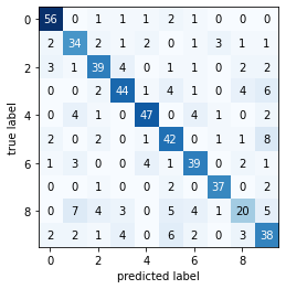
Computing a confusion matrix and obtaining our model accuracy…
print('Scikit-learn Decision Tree Classifier on digits dataset... \n')
print('-'*10 + 'Classification Report' + '-'*5)
print(metrics.classification_report(y_test, y_pred))
print('-'*10 + 'Confusion Matrix' + '-'*10)
plot_confusion_matrix(metrics.confusion_matrix(y_test, y_pred))
Scikit-learn Decision Tree Classifier on digits dataset...

----------Classification Report-----
              precision    recall  f1-score   support

           0       0.98      0.94      0.96        64
           1       0.78      0.75      0.76        52
           2       0.93      0.85      0.89        67
           3       0.84      0.87      0.85        53
           4       0.80      0.90      0.85        41
           5       0.94      0.82      0.88        57
           6       0.86      0.91      0.88        46
           7       0.91      0.84      0.88        58
           8       0.68      0.81      0.74        52
           9       0.77      0.80      0.78        50

    accuracy                           0.85       540
   macro avg       0.85      0.85      0.85       540
weighted avg       0.86      0.85      0.85       540

----------Confusion Matrix----------
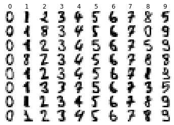
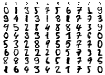
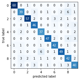 Great, we’ve classified our test set images using the fitted decision tree. As we saw in the confusion matrix, our model wasn’t perfect. We notice some misclassifications, especially with the
 1 and 8 digit images. The following code will let us display a random sample of test images and their predicted labels.
def visualize_predictions(images, labels, examples_per_class):
    """
    Display a sample of randomly selected images and their predicted labels
    """
    #images_and_predictions = list(zip(images, labels))
    number_of_classes = len(np.unique(labels))
    for cls in range(number_of_classes):
        idxs = np.where(labels == cls)[0]
        idxs = np.random.choice(idxs, examples_per_class, replace=False)
        for i, idx in enumerate(idxs):
            plt.subplot(examples_per_class, number_of_classes, i * number_of_classes + cls + 1)
            plt.imshow(images[idx].astype('uint8'), cmap=plt.cm.gray_r, interpolation='nearest')
            plt.axis('off')
            if i == 0:
                plt.title('%s' % str(cls))
    plt.show()
# Reshape test data to 3D
X_test_images = X_test.reshape((len(X_test),8,8))
visualize_predictions(X_test_images, y_pred, examples_per_class=8)
In the next section, we will modify a few of the DecisionTreeClassifier parameters and see if we can optimise our model.
Modifying the Scikit-learn DecisionTreeClassifier
5. Change the parameters of the classifier, e.g., the minimum number of samples in a leaf / for a split, to see how the tree and the results are affected.
Parameters modified:
criterion: specifies the function to use to measure the quality of a split.
We’ll first modify the Scikit-learn DecisionTreeClassifier by setting our splitting criterion (the function that measures discriminatory power) to entropy. This allows us to calculate information gain for each attribute rather than the Scikit-learn default of Gini impurity. The resulting classifier’s performance can be compared to our own ID3-algorithm we will be coding from scratch, which also uses information gain as its splitting criterion. This will be covered in the later part of the notebook. For now, let’s see how our results with the DecisionTreeClassifier are impacted by this change.
# Using information gain to determine best split
classifier = tree.DecisionTreeClassifier(criterion='entropy')
# Fitting decision tree on training set
id3esqueTree = classifier.fit(X_train, y_train)
# Visualising the new tree
plt.figure(figsize=(20,20))
tree.plot_tree(id3esqueTree)
plt.show()
# Predicting over test set
y_pred = id3esqueTree.predict(X_test)
print('Scikit-learn Decision Tree Classifier (using information gain) on digits dataset... \n')
print('-'*10 + 'Classification Report' + '-'*5)
print(metrics.classification_report(y_test, y_pred))
print('-'*10 + 'Confusion Matrix' + '-'*10)
plot_confusion_matrix(metrics.confusion_matrix(y_test, y_pred))
Scikit-learn Decision Tree Classifier (using information gain) on digits dataset...

----------Classification Report-----
              precision    recall  f1-score   support

           0       0.97      0.95      0.96        64
           1       0.81      0.83      0.82        52
           2       0.90      0.82      0.86        67
           3       0.87      0.87      0.87        53
           4       0.73      0.85      0.79        41
           5       0.89      0.82      0.85        57
           6       0.90      0.96      0.93        46
           7       0.82      0.72      0.77        58
           8       0.71      0.75      0.73        52
           9       0.78      0.84      0.81        50

    accuracy                           0.84       540
   macro avg       0.84      0.84      0.84       540
weighted avg       0.84      0.84      0.84       540

----------Confusion Matrix----------
Great, we now have a reasonable model to compare to later on when we’ve constructed our own ID3-algorithm. Before we jump into writing our code, let’s try one more modification to the Scikit-learn DecisionTreeClassifier. The parameters that we will modify below are rather difficult to implement in our own version, so it’s best to test them out now.
Parameters modified:
max_depth: the maximum depth of the tree (default is until all nodes are leaves).min_samples_split: the minimum number of samples to split an internal node.min_samples_leaf: the minimum number of samples required to be at a leaf node.
There are a few reasons why we would want to modify the above parameters in practice. Let’s start with max_depth. The theoretical maximum depth of a decision tree is one less than the number of samples in the training set. A decision tree with this depth is, however, undesirable. The deeper the tree grows, the more complex the model becomes. The more attribute splits there are, the higher than chance of overfitting of the training data. Thus, reducing the maximum depth of the decision tree is one way to prevent overfitting.
def test_depth(X_train, X_test, y_train, y_test, max_depth=10):
    """
    Calculates the average F1 score over ten training runs for each model variation.
    Each model is tested with a max_depth from 10 to max_depth, inclusive.
    """
    f1_scores = {}
    for i in range(10, max_depth+1):
        f1s = []
        for exp in range(10):
            model = tree.DecisionTreeClassifier(max_depth=i)
            model.fit(X_train, y_train)
            y_pred = model.predict(X_test)
            # Multi-class F1 requires 'macro' or 'weighted' average
            # We choose 'macro' as our training set is relatively balanced
            f1s.append(metrics.f1_score(y_test, y_pred, average='macro'))
        f1_scores[i] = np.mean(f1s)
    return f1_scores
f1_scores = test_depth(X_train, X_test, y_train, y_test, max_depth=20)
f1_scores
{10: 0.8491836659477479,
 11: 0.8540618473168712,
 12: 0.8506428083925082,
 13: 0.8484501993680255,
 14: 0.8476100596481668,
 15: 0.8525831603915026,
 16: 0.8497516840174912,
 17: 0.8536172826836271,
 18: 0.8506231543841205,
 19: 0.8525277761148755,
 20: 0.8519916298862185}
plt.figure()
plt.plot(list(f1_scores.keys()), list(f1_scores.values()))
plt.title('Average F1 scores')
plt.xlabel('max_depth')
plt.ylabel('F1 score')
plt.show()
# Get max_depth of model with highest average F1 score
best_depth = max(f1_scores, key=lambda x: f1_scores[x])
best_depth
11
To find the best performing model, we will use Scikit-learn’s GridSearchCV. This handy method allows us to test each hyperparameter combination on a given classifier and find the best combination from the parameter grid we specified. This works by exhaustively searching the parameter space using cross-validation method. One limitation to this approach is that we have to manually set a range of values to try for each hyperparameter. To better determine this, consult a research paper that uses a similar model and dataset. We chose our value ranges from the recommendations in this blog post on tuning decision trees.
from sklearn.model_selection import GridSearchCV
# Parameters to test (see above)
params = {'max_depth': range(10,21),
          'min_samples_split': range(1,41),
          'min_samples_leaf': range(1,21)}
# Perform cross-validated grid-search over parameter grid
grid = GridSearchCV(tree.DecisionTreeClassifier(),
                    # Parameters and their values to test in dict format
                    param_grid=params,
                    # Cross-validation method (int=k folds for KFold)
                    cv=10,
                    # Number of jobs to run in parallel (-1 uses all processors)
                    n_jobs=-1,
                    # Print computation time for each fold and parameter candidate
                    verbose=1,
                    # Include training scores in cv_results_
                    return_train_score=True)
Forewarning: running GridSearchCV could take quite a long time (up to 15 minutes, in our case). Make sure that you have a decent computer or access to one. Google Colab provides a great (and free!) cloud service that handles this task fairly well.
# Perform the grid search and fit on training data
grid.fit(X_train, y_train)
Fitting 10 folds for each of 8800 candidates, totalling 88000 fits

[Parallel(n_jobs=-1)]: Using backend LokyBackend with 2 concurrent workers.
[Parallel(n_jobs=-1)]: Done 230 tasks      | elapsed:    3.6s
[Parallel(n_jobs=-1)]: Done 1430 tasks      | elapsed:   17.0s
[Parallel(n_jobs=-1)]: Done 3430 tasks      | elapsed:   38.4s
[Parallel(n_jobs=-1)]: Done 6230 tasks      | elapsed:  1.1min
[Parallel(n_jobs=-1)]: Done 9830 tasks      | elapsed:  1.7min
[Parallel(n_jobs=-1)]: Done 14230 tasks      | elapsed:  2.5min
[Parallel(n_jobs=-1)]: Done 19430 tasks      | elapsed:  3.4min
[Parallel(n_jobs=-1)]: Done 25430 tasks      | elapsed:  4.5min
[Parallel(n_jobs=-1)]: Done 32230 tasks      | elapsed:  5.6min
[Parallel(n_jobs=-1)]: Done 39830 tasks      | elapsed:  7.0min
[Parallel(n_jobs=-1)]: Done 48230 tasks      | elapsed:  8.5min
[Parallel(n_jobs=-1)]: Done 57430 tasks      | elapsed: 10.1min
[Parallel(n_jobs=-1)]: Done 67430 tasks      | elapsed: 11.9min
[Parallel(n_jobs=-1)]: Done 78230 tasks      | elapsed: 13.7min
[Parallel(n_jobs=-1)]: Done 88000 out of 88000 | elapsed: 15.4min finished
The following returns the combination of hyperparameter values that gave us the best results.
# Parameter setting that gave the best results
grid.best_params_
{'max_depth': 13, 'min_samples_leaf': 1, 'min_samples_split': 2}
It looks like our best max_depth value has changed slightly. Interestingly, the best reported values for min_samples_leaf and min_samples_split are the default ones in scikit-learn. Let’s see how the classifier performed with the hyperparameter combination…
# Mean cross-validated score of the best estimator
grid.best_score_
0.8767365079365079
Not bad! It looks like a bit of hyperparameter tuning was able to improve the stock DecisionTreeClassifier accuracy by several percentage points. Don’t get too excited, though. We have to still perform our train-test routine with this hyperparameter combination to get a better idea of the true predictive performance of the model. GridSearchCV only reports the mean cross-validated “score” during training and does not evaluate the performance on a test set.
Each parameter’s performance is returned in a nested dictionary object. Using the following method, we can visualise the mean score of each hyperparameter value.
from plotly.subplots import make_subplots
import plotly.graph_objects as go
import plotly.io as pio
def plot_search_results_plotly(grid):
    """
    Plot the mean scores per parameter evaluated with GridSearchCV.

    Params:
        grid: trained GridSearchCV object
    """
    # GridSearchCV results
    results = grid.cv_results_
    means_test = results['mean_test_score']
    stds_test = results['std_test_score']
    means_train = results['mean_train_score'] #
    stds_train = results['std_train_score'] #

    # Indices of hyperparameters
    masks = []
    mask_names = list(grid.best_params_.keys())
    for p_k, p_v in grid.best_params_.items():
        masks.append(list(results['param_'+p_k].data==p_v))
    params = grid.param_grid

    # Best parameter values
    best_values = grid.best_params_

    # Display results with Plotly
    fig = make_subplots(rows=1, cols=len(params), subplot_titles=mask_names, shared_xaxes=False, shared_yaxes=True)
    for i, p in enumerate(mask_names):
        m = np.stack(masks[:i] + masks[i+1:])
        best_params_mask = m.all(axis=0)
        best_index = np.where(best_params_mask)[0]
        x = np.array(params[p])
        y_1 = np.array(means_test[best_index])
        e_1 = np.array(stds_test[best_index])
        y_2 = np.array(means_train[best_index]) #
        e_2 = np.array(stds_train[best_index])  #
        fig.add_trace(go.Scatter(x=x, y=y_1, error_y=dict(type='data', array=e_1), legendgroup="test_group", name='test'), row=1, col=i+1)
        fig.add_trace(go.Scatter(x=x, y=y_2, error_y=dict(type='data', array=e_2), legendgroup="train_group", name='train'), row=1, col=i+1) #
    fig.update_layout(title_text='Scores per parameter for DecisionTreeClassifier', showlegend=True)
    fig.update_yaxes(title_text='Mean score', row=1, col=1)
    fig.show()
    pio.write_html(fig, file='cv_scores.html', auto_open=True)
plot_search_results_plotly(grid)
import joblib

# Save the GridSearchCV object
joblib.dump(grid, 'grid_search_cv.pkl')
best_classifier = tree.DecisionTreeClassifier(**grid.best_params_)
best_classifier
DecisionTreeClassifier(ccp_alpha=0.0, class_weight=None, criterion='gini',
                       max_depth=13, max_features=None, max_leaf_nodes=None,
                       min_impurity_decrease=0.0, min_impurity_split=None,
                       min_samples_leaf=1, min_samples_split=2,
                       min_weight_fraction_leaf=0.0, presort='deprecated',
                       random_state=None, splitter='best')
best_sklearnTree = best_classifier.fit(X_train, y_train)
# Visualise the modified tree
plt.figure(figsize=(30,30))
tree.plot_tree(best_sklearnTree)
plt.show()
y_pred = best_sklearnTree.predict(X_test)
print('Scikit-learn Decision Tree Classifier (with modified parameters) on digits dataset... \n')
print('classifier: %s\n' % best_classifier)
print('-'*10 + 'Classification Report' + '-'*5)
print(metrics.classification_report(y_test, y_pred))
print('-'*10 + 'Confusion Matrix' + '-'*10)
plot_confusion_matrix(metrics.confusion_matrix(y_test, y_pred))
Scikit-learn Decision Tree Classifier (with modified parameters) on digits dataset...

classifier: DecisionTreeClassifier(ccp_alpha=0.0, class_weight=None, criterion='gini',
                       max_depth=13, max_features=None, max_leaf_nodes=None,
                       min_impurity_decrease=0.0, min_impurity_split=None,
                       min_samples_leaf=1, min_samples_split=2,
                       min_weight_fraction_leaf=0.0, presort='deprecated',
                       random_state=None, splitter='best')

----------Classification Report-----
              precision    recall  f1-score   support

           0       0.98      0.94      0.96        64
           1       0.77      0.85      0.81        52
           2       0.93      0.85      0.89        67
           3       0.81      0.87      0.84        53
           4       0.80      0.90      0.85        41
           5       0.92      0.82      0.87        57
           6       0.84      0.91      0.87        46
           7       0.96      0.78      0.86        58
           8       0.70      0.83      0.76        52
           9       0.82      0.80      0.81        50

    accuracy                           0.85       540
   macro avg       0.85      0.85      0.85       540
weighted avg       0.86      0.85      0.86       540

----------Confusion Matrix----------

2. Decision Tree Classifier using the ID3 algorithm
Objective #2: Implementing our own decision tree classifier based on the ID3 algorithm…
In the first part of this article, we framed classification as a kind of questioning-answering problem. We discussed how a decision tree naturally structures this type of hierarchial decision-making system. We then introduced the basic idea of the decision tree algorithm and lightly covered the general strategy of recursively building subtrees by splitting data into subsets based on an optimal attribute. To demonstrate this process, we applied a Scikit-learn DecisionTreeClassifier (implemented with CART) to the digits dataset. We saw what the resulting tree structure looked like, then measured its performance by classifying the test data subset. Lastly, we tuned a few hyperparameters like max_depth, which acts to minimise the depth of the tree (the number of ‘questions’ asked).
In this section, we will write our own algorithm from scratch, following the same general algorithm for decision trees we saw earlier. However, in our implementation we will be modifying the splititng criterion to follow the ID3 (Iterative Dichotomiser 3) algorithm. To review, the splitting criterion is a function used to measure which ‘questions’ provide the most value when it comes to separating the data. The ID3 algorithm selects the most useful attributes by introducing a metric known as information gain.
Information gain determines which questions (attributes) have the ‘most value’ by calculating their respective entropy reduction in terms of Shannon entropy. We can express this entropy calculation for a given discrete random variable \(X\) as \(H(X)\). At the highest level, information gain \(IG(T,a)\) can then be thought of as simple difference formula between the a prior Shannon entropy \(H(T)\) of data set \(T\) and the conditional entropy \(H(T\mid a)\) after splitting that dataset on attribute \(a\). Thus, information gain is expressed as


Given a discrete random variable \(X\) with possible outcomes \(x_{1},...,x_{n}\), which occur with probability \(P(x_{1}),...,P(x_{n})\), we can then define the Shannon entropy \(H(X)\) to be

where \(\sum\) denotes the sum over the variable’s possible values. In our application, we will be choosing \(log\) to be of Base 2 with units of bits as “shannons”.
To build our decision tree branch-by-branch, we perform the above calculations in a four-step process at each recursive call:
- Calculate the prior entropy of the data set.
- Calculate the information gain for each attribute.
- Select the attribute with the maximal information gain.
- Partition the dataset based on the best attribute’s values.
Like the CART decision tree algorithm we covered in the first section of this article, we stop performing the above when any of the following conditions are met:
- There are no remaining samples to split, or
- There are no remaining attributes to split on (all samples are of the same class).
The ID3 algorithm in pseudocode
ID3 (Samples, Target_Attribute, Attributes)
  Create a (root) node Root for the tree

  If all samples belong to one class <class_name>
      Return the single-node tree Root, with label = <class_name>.

  If Attributes is empty, then
      Return the single node tree Root, with label = most common class value in Samples.
  else
      Begin
          Let A be the attribute a in Attributes that generates the maximum information gain
                when the tree is split based on a.

          Set A as the target_attribute of Root

          For each possible value, v, of A, add a new tree branch below Root,
               corresponding to the test A == v, i.e.,
              Let Samples(v) be the subset of samples that have the value v for A.
              If Samples(v) is empty, then
                  Below this new branch add a leaf node with label
                        = most common class value in Samples.
              else
                  Below this new branch add the subtree ID3 (Samples(v), A, Attributes/{A})
        End
  Return Root
1. Make a decision regarding the data structure that your tree should be able to handle. In the code below, you will find the tree assumed to be implemented with nodes that are dictionaries.
We will be using the Handout_SkeletonDT code provided to us by E.A. Topp (EDAN95, link here) to help us get started on our ID3 decision tree algorithm. Examine the ID3DecisionTreeClassifierSkeleton class a bit to understand how we will implement nodes and visualise them in a graph using the pydot library.
from collections import Counter
from graphviz import Digraph


class ID3DecisionTreeClassifierSkeleton:


    def __init__(self, minSamplesLeaf = 1, minSamplesSplit = 2):

        self.__nodeCounter = 0

        # the graph to visualise the tree
        self.__dot = Digraph(comment='The Decision Tree')

        # suggested attributes of the classifier to handle training parameters
        self.__minSamplesLeaf = minSamplesLeaf
        self.__minSamplesSplit = minSamplesSplit


    # Create a new node in the tree with the suggested attributes for the visualisation.
    # It can later be added to the graph with the respective function
    def new_ID3_node(self):
        node = {'id': self.__nodeCounter, 'label': None, 'attribute': None, 'entropy': None, 'samples': None,
                         'classCounts': None, 'nodes': None}

        self.__nodeCounter += 1
        return node

    # adds the node into the graph for visualisation (creates a dot-node)
    def add_node_to_graph(self, node, parentid=-1):
        nodeString = ''
        for k in node:
            if ((node[k] != None) and (k != 'nodes')):
                nodeString += "\n" + str(k) + ": " + str(node[k])

        self.__dot.node(str(node['id']), label=nodeString)
        if (parentid != -1):
            self.__dot.edge(str(parentid), str(node['id']))
            nodeString += "\n" + str(parentid) + " -> " + str(node['id'])

        print(nodeString)

        return


    # make the visualisation available
    def make_dot_data(self):
        return self.__dot


    # For you to fill in; Suggested function to find the best attribute to split with, given the set of
    # remaining attributes, the currently evaluated data and target.
    def find_split_attr(self):

        # Change this to make some more sense
        return None


    # the entry point for the recursive ID3-algorithm, you need to fill in the calls to your recursive implementation
    def fit(self, data, target, attributes, classes):

        # fill in something more sensible here... root should become the output of the recursive tree creation
        root = self.new_ID3_node()
        self.add_node_to_graph(root)

        return root


    def predict(self, data, tree):
        predicted = list()

        # fill in something more sensible here... root should become the output of the recursive tree creation
        return predicted
2. Inspect other parts of the code provided. You will find one example for how it is easily possible to construct the visualisation data (dot-data) for the graphviz-visualisation in parallel to the actual decision tree. Whenever a node is added to the tree, it can also immediately be added to the graph. Feel free to use this for your own implementation.
In the above implementation we visualise our decision tree by calling the make_dot_data() method on a tree object that has been fitted (trained). We then wish to save a PDF of the visualised tree, which we can do by calling render() and passing in a desired filename.
# Initialise the decision tree model
clf = ID3()
# Fit on training data (build tree)
example_tree = clf.fit(train_data, train_labels)
# Construct pydot-node visualisation
plot = example_tree.make_dot_data()
# Save to PDF
plot.render("testTree")
In order to implement the desired functionality above, we need to install a few dependencies.
# Render PDF in image format to display tree inline
!pip install pdf2image
Collecting pdf2image
  Downloading pdf2image-1.16.0-py3-none-any.whl (10 kB)
Requirement already satisfied: pillow in /usr/local/lib/python3.7/dist-packages (from pdf2image) (7.1.2)
Installing collected packages: pdf2image
Successfully installed pdf2image-1.16.0
# Install poppler dependency
!apt-get install poppler-utils
Reading package lists... Done
Building dependency tree
Reading state information... Done
The following NEW packages will be installed:
  poppler-utils
# Check if poppler was installed successfully
!pdftoppm -h
pdftoppm version 0.62.0
Copyright 2005-2017 The Poppler Developers - http://poppler.freedesktop.org
Copyright 1996-2011 Glyph & Cog, LLC
Below is a method to display an image from a PDF in a Jupyter notebook cell.
from pdf2image import convert_from_path
from pathlib import Path
from PIL import Image
import matplotlib.pyplot as plt

def display_tree(filename):
    path = Path(filename)
    img_name = path.with_suffix('')
    pages = convert_from_path(path, dpi=200)

    for idx,page in enumerate(pages):
        img_path = Path(str(img_name) + '_page' + str(idx)).with_suffix('.jpg')
        page.save(img_path, 'JPEG')
        plt.figure()
        plt.title(img_name)
        img = Image.open(img_path)
        plt.imshow(img)
        plt.axis('off')
        plt.show()
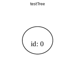
3. Simply running main in the handout will produce a tree with one node, visualised in testTree.pdf. Make sure that this works, i.e., that you have all the necessary libraries installed.
In order to test our decision tree, we will first use a rather simple toy dataset. This dataset is split into attributes, classes, target and data. A description of each follows:
attributes: list of tuples in the form(attribute_name, [list, of, attribute, values])classes: tuple of the unique classes (positive or negative)data: list of training examples as tuples that contain the respective attribute values for each unique attribute inattributestarget: tuple of class labels for each example indatatestData: list of test examples as tuples that contain the respective attribute values for each unique attribute inattributestestTarget: tuple of class labels for each example intestData
### From `ToyData.py` in E.A. Topp's `Handout_SkeletonDT`
from collections import OrderedDict

class ToyData:

    def __init__(self):
        self.attributes = OrderedDict(
            [("color", ["y", "g", "b"]), ("size", ["s", "l"]), ("shape", ["r", "i"])]
        )
        self.classes = ('+', '-')

        self.data = [('y', 's', 'r'),
                 ('y', 's', 'r'),
                 ('g', 's', 'i'),
                 ('g', 'l', 'i'),
                 ('y', 'l', 'r'),
                 ('y', 's', 'r'),
                 ('y', 's', 'r'),
                 ('y', 's', 'r'),
                 ('g', 's', 'r'),
                 ('y', 'l', 'r'),
                 ('y', 'l', 'r'),
                 ('y', 'l', 'r'),
                 ('y', 'l', 'r'),
                 ('y', 'l', 'r'),
                 ('y', 's', 'i'),
                 ('y', 'l', 'i')]
        self.target = ('+', '-', '+', '-', '+', '+', '+', '+', '-', '-', '+', '-', '-', '-', '+', '+')

        self.testData = [('y', 's', 'r'),
                 ('y', 's', 'r'),
                 ('g', 's', 'i'),
                 ('b', 'l', 'i'),
                 ('y', 'l', 'r')]

        self.testTarget = ('+', '-', '+', '-', '+')

    def get_data(self):
        return self.attributes, self.classes, self.data, self.target, self.testData, self.testTarget
As mentioned in Step 3, running the following code should produce a decision tree that contains a single node with id: 0. Nothing interesting can be said just yet about the resulting tree, but our goal is rather to test that our visualisation libraries are properly installed.
### From `main.py` in E.A. Topp's `Handout_SkeletonDT`
#import ToyData as td
#import ID3

import numpy as np
from sklearn import tree, metrics, datasets


def main():
	# Get data from ToyData
    attributes, classes, data, target, data2, target2 = ToyData().get_data()
    # Initialise decision tree model
    id3_test = ID3DecisionTreeClassifierSkeleton()
    # Fit the decision tree on ToyData (build tree)
    myTree = id3_test.fit(data, target, attributes, classes)
    print(myTree)
    # Visualise nodes using pydot
    plot = id3_test.make_dot_data()
    # Save to PDF
    plot.render("testTree")
    # Run a "prediction" over the test data
    predicted = id3_test.predict(data2, myTree)
    print(predicted)


if __name__ == "__main__": main()
# Visualise the tree and verify that a single node is produced
display_tree('testTree.pdf')
The ID3 Decision Tree Classifier
4. The code handout contains a mere skeleton for the ID3 classifier. Implement what is needed to actually construct a decision tree classifier. Implement the ID3 algorithm, e.g., according to what is provided in the lecture or on this page below. Use information gain as criterion for the best split attribute.
Now, the moment we have been waiting for. It’s finally time to write our very own ID3 Decision Tree Classifier. Follow the code below and you’ll be up and running in no time. The code is heavily documented with plenty of comments to help guide you through the implementation from top to bottom.
from collections import Counter, OrderedDict
from graphviz import Digraph
import math

class ID3DecisionTreeClassifier:
    def __init__(self, minSamplesLeaf = 1, minSamplesSplit = 2) :
        # The number of nodes in the tree
        self.__nodeCounter = 0
        # The graph to visualise the tree
        self.__dot = Digraph(comment='The Decision Tree')
        # Suggested attributes of the classifier to handle training parameters
        self.__minSamplesLeaf = minSamplesLeaf
        self.__minSamplesSplit = minSamplesSplit

    def new_ID3_node(self):
        """
        Create a new node in the tree with the suggested attributes for the visualisation.
        It can later be added to the graph with the respective function
        """
        # The node object implemented with a dictionary
        node = {'id': self.__nodeCounter, 'label': None, 'attribute': None, 'entropy': None, 'samples': None,
                         'classCounts': None, 'nodes': None}

        # New key to store parent node's attribute value
        node.update({'attribute_value': None})
        # Incremement the counter by one for every new node created
        self.__nodeCounter += 1
        return node

    def add_node_to_graph(self, node, parentid=-1):
        """
        Create a dot-node for visualisation and print the node
        """
        nodeString = ''
        for k in node:
            if ((node[k] != None) and (k != 'nodes')):
                nodeString += "\n" + str(k) + ": " + str(node[k])

        self.__dot.node(str(node['id']), label=nodeString)
        if (parentid != -1):
            self.__dot.edge(str(parentid), str(node['id']))
            nodeString += "\n" + str(parentid) + " -> " + str(node['id'])

        print(nodeString)
        return


    # make the visualisation available
    def make_dot_data(self):
        return self.__dot

    def _calc_entropy(self, node):
        """
        Return the entropy score of the data set prior to splitting.
        """
        entropy = 0.0
        # If all targets are of the same class, the entropy value is 0
        if len(node['classCounts'].values()) == 1:
            return entropy
        # Compute the weighted sum of the log of the probabilities
        for count in node['classCounts'].values():
            prob = count / node['samples']
            entropy -= prob * math.log2(prob)
        self._entropy = entropy
        return self._entropy

    def _calc_information_gain(self, target, attributes, node):
        """
        Returns the information gain of each attribute in attributes.
        Information gain is measured as the difference in entropy values calculated
        before and after the split on the most optimal attribute.
        """
        info_gain = 0
        # Store information gain for each remaining attribute in attributes
        information_gains = {}
        for attribute in attributes:
            # Get entropy of parent node
            info_gain = node['entropy']
            # Store weighted average entropy
            weighted_entropy = 0.0
            # For every attribute value and its indexes in target
            for attribute_value, attribute_idxs in attributes[attribute].items():
                if attribute_idxs:
                    # Get the class labels of the attribute value by index
                    attribute_value_targets = {i:target[i] for i in attribute_idxs if i in target.keys()}
                    # Store the frequencies of each class label
                    classCounts = Counter(attribute_value_targets.values())
                    # Calculate the entropy of each child
                    child_entropy = 0.0
                    for count in classCounts.values():
                        prob = count / len(attribute_value_targets)
                        child_entropy -= prob * math.log2(prob)
                    # Calculate the weighted average entropy score if we were to split at this attribute
                    weighted_entropy += (len(attribute_value_targets) / node['samples']) * child_entropy
                    # Update summed info gain score for this attribute value
                    info_gain -= weighted_entropy
            # Update total information gain for this attribute
            information_gains[attribute] = info_gain
        self._information_gains = information_gains
        return self._information_gains

    def _get_best_split(self, target, attributes, node):
        """
        Returns the attribute that has the most predictive power (yields the most information if the data set was split based on that attribute's values).
        This attribute has the highest information gain.
        """
        info_gains = self._calc_information_gain(target, attributes, node)
        best_split = max(info_gains, key=lambda x: info_gains[x])

        self._best_split = best_split
        return self._best_split


    def build_tree(self, data, target, attributes, classes, attr_val="", parentid=-1):
        """
        The recursive ID3-algorithm. On each iteration, the entropy and information gain of each attribute is calculated. In summary,
           1. Calculate the entropy of every attribute in attributes.
           2. Split the data into subsets using the attribute whose resulting information gain is maximised.
           3. Create a decision tree node using that attribute.
           4. Recursively perform steps 1-3 until the stopping conditions are satisfied.
        """
        # Count the frequencies of each class in target
        classCounts = Counter(target.values())

        # Create new node and update its values
        node = self.new_ID3_node()
        node.update({'samples': len(data)})
        node.update({'classCounts': classCounts})
        node.update({'entropy': self._calc_entropy(node)})
        node.update({'attribute_value': attr_val})

        # Create an empty list to store child nodes
        children = []

        # Stopping condition: no remaining attributes to split on
        if not attributes:
            # Update label of leaf node to be the name of the most frequent class
            # n=1 ensures that we return only the most common element in target
            # [0][0] ensures that we return the label rather than count
            node.update({'label': classCounts.most_common(1)[0][0]})
            # Add the node into the graph for visualisation
            self.add_node_to_graph(node, parentid)
            return node
        # Stopping condition: all samples in target are of the same class
        elif len(classCounts) == 1:
            # Update label of leaf node to be the name of the most frequent class
            node.update({'label': classCounts.most_common(1)[0][0]})
            # Add the node into the graph for visualisation
            self.add_node_to_graph(node, parentid)
            return node
        else:
            # Get the attribute to split on whose values have the highest information gain
            best_attribute = self._get_best_split(target, attributes, node)
            node.update({'attribute': best_attribute})
            # Add the node into the graph for visualisation
            self.add_node_to_graph(node, parentid)
            best_attribute_dict = attributes[best_attribute]

            # Recursively build branches by computing the best remaining attributes to split on
            for attribute_value, attribute_value_idxs in best_attribute_dict.items():
                # Remove the split attribute
                attributes_partitioned = attributes.copy()
                attributes_partitioned.pop(best_attribute, None)
                # Get the samples from data by index that contain the attribute value
                data_partitioned = {idx:data[idx] for idx in attribute_value_idxs if idx in data.keys()}
                # Get the class labels from target that map to the attribute value pairs
                target_partitioned = {idx:target[idx] for idx in attribute_value_idxs if idx in target.keys()}

                # If there are remaining attribute values to split
                if data_partitioned:
                    # Call recursive function to find the next best attribute(s) to split on
                    child = self.build_tree(data_partitioned, target_partitioned, attributes_partitioned, classes, attribute_value, node['id'])
                    # Append the new child node to the list of children
                    children.append(child)
                else:
                    # Create a leaf node
                    child = self.new_ID3_node()
                    # Update leaf node values
                    child.update({'label': classCounts.most_common(1)[0][0]})
                    child.update({'samples': len(attribute_value_idxs)})
                    #child.update({'samples': 0})
                    child.update({'attribute_value': attribute_value})
                    # Add the leaf node into the graph for visualisation
                    self.add_node_to_graph(child, node['id'])
                    children.append(child)

            node.update({'nodes': children})
        return node

    def fit(self, data, target, attributes, classes, dataset=""):
        """
        The entry point for the recursive ID3-algorithm. Formats the input data and returns a root to the decision tree.
        """
        # Format the Scikit-learn digits dataset
        if dataset is not "ToyData":
            # Assume attributes is a list with the unique values of all attributes in data
            # Append the list of values as a tuple to every index in the list whose length is equal to the number of attributes in data
            attributes = [tuple(attributes) for i in range(data.shape[1])]
            # Create a dict of attribute values indexed by the number of attributes in data
            attributes = OrderedDict(zip(range(data.shape[1]), attributes))
            # Convert each sample in data (a list of attribute values) to a tuple and store it in a list
            data = [tuple(x) for x in data]
            # Convert the target labels into a tuple
            target = tuple(target)

        # Index the input data
        data_indexed = {i:data[i] for i in range(len(data))}
        target_indexed = {i:target[i] for i in range(len(target))}
        attributes_indexed = {attr:i for i, attr in enumerate(attributes.keys())}

        # Build nested attribute dict where each attribute value is paired with the indices in data where it occurs
        for i, attribute in enumerate(attributes.keys()):
            # Get the list of attribute values
            attribute_values = attributes[attribute]
            # Build dict to store each attribute value and an empty list for its indices in the data
            attribute_value_idx = {attribute_value:[] for attribute_value in attribute_values}
            # Go through each sample in the data
            for idx, x in data_indexed.items():
                # Get the value of the ith attribute in the sample
                x_value = x[i]
                # Append the sample's index to its matching attribute value in the dict
                attribute_value_idx[x[i]].append(idx)
            # Save the attribute's value-indicies mapping
            attributes[attribute] = attribute_value_idx

        # Build the decision tree using the ID3-algorithm and return its root node
        root = self.build_tree(data_indexed, target_indexed, attributes, classes)

        self._attributes_indexed = attributes_indexed
        self._root = root
        return self._root

    def _predict(self, x, node):
        """
        Helper function to predict the class label of a single instance in the test set by traversing the decision tree until a matching leaf node is found.
        """
        # The leaf node
        if node['label'] is not None:
            # Return its label as the predicted class for sample x
            return node['label']
        # The entry point into the tree traversal
        else:
            # Get the best split attribute at the current node
            best_attribute = node['attribute']
            # Return the value in the sample that belongs to the current split attribute
            attribute_value = x[self._attributes_indexed[best_attribute]]
            # Traverse through the branches
            for child in node['nodes']:
                # If the attribute value is found in the child node (a leaf)
                if attribute_value == child['attribute_value']:
                    # Call the method to return the leaf node label
                    return self._predict(x, child)

    def predict(self, data, tree, dataset=""):
        """
        Predicts the class labels of the test set sample-by-sample by traversing the decision tree built during training.
        """
        predicted = list()

        # Format the dataset
        if dataset is not "ToyData":
            data = [tuple(x) for x in data]
        for x in data:
            # Append the predicted label of x to the list
            predicted.append(self._predict(x, tree))

        self.y_pred = predicted
        return self.y_pred
5. Test your classifier with the toy example provided in the ToyData class given in the skeleton. In main you can also see how to make use of the dot-data to produce a visualisation with graphviz.
Ready to run our very own decision tree algorithm through some data? Let’s go!
# Get data from ToyData
attributes, classes, data, target, data2, target2 = ToyData().get_data()
# Initialise decision tree model
id3 = ID3DecisionTreeClassifier()
# Fit on training data (build tree)
toyTree = id3.fit(data, target, attributes, classes)
id: 0
attribute: size
entropy: 0.9886994082884974
samples: 16
classCounts: Counter({'+': 9, '-': 7})
attribute_value:

id: 1
attribute: color
entropy: 0.8112781244591328
samples: 8
classCounts: Counter({'+': 6, '-': 2})
attribute_value: s
0 -> 1

id: 2
attribute: shape
entropy: 0.6500224216483541
samples: 6
classCounts: Counter({'+': 5, '-': 1})
attribute_value: y
1 -> 2

id: 3
label: +
entropy: 0.7219280948873623
samples: 5
classCounts: Counter({'+': 4, '-': 1})
attribute_value: r
2 -> 3

id: 4
label: +
entropy: 0.0
samples: 1
classCounts: Counter({'+': 1})
attribute_value: i
2 -> 4

id: 5
attribute: shape
entropy: 1.0
samples: 2
classCounts: Counter({'+': 1, '-': 1})
attribute_value: g
1 -> 5

id: 6
label: -
entropy: 0.0
samples: 1
classCounts: Counter({'-': 1})
attribute_value: r
5 -> 6

id: 7
label: +
entropy: 0.0
samples: 1
classCounts: Counter({'+': 1})
attribute_value: i
5 -> 7

id: 8
label: +
samples: 0
attribute_value: b
1 -> 8

id: 9
attribute: shape
entropy: 0.9544340029249649
samples: 8
classCounts: Counter({'-': 5, '+': 3})
attribute_value: l
0 -> 9

id: 10
attribute: color
entropy: 0.9182958340544896
samples: 6
classCounts: Counter({'-': 4, '+': 2})
attribute_value: r
9 -> 10

id: 11
label: -
entropy: 0.9182958340544896
samples: 6
classCounts: Counter({'-': 4, '+': 2})
attribute_value: y
10 -> 11

id: 12
label: -
samples: 3
attribute_value: g
10 -> 12

id: 13
label: -
samples: 0
attribute_value: b
10 -> 13

id: 14
attribute: color
entropy: 1.0
samples: 2
classCounts: Counter({'-': 1, '+': 1})
attribute_value: i
9 -> 14

id: 15
label: +
entropy: 0.0
samples: 1
classCounts: Counter({'+': 1})
attribute_value: y
14 -> 15

id: 16
label: -
entropy: 0.0
samples: 1
classCounts: Counter({'-': 1})
attribute_value: g
14 -> 16

id: 17
label: -
samples: 0
attribute_value: b
14 -> 17
# Visualise nodes using pydot
plot = id3.make_dot_data()
# Save to PDF
plot.render('myToyTree')
'myToyTree.pdf'
# Display PDF of tree inline
display_tree('myToyTree.pdf')
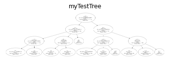
We successfully fit a decision tree on the ToyData dataset using our very own ID3 algorithm! In essence, our algorithm has figured out which ‘questions’ to ask about the attribute value pairs in the test data to identify whether or not a given example is either positive (+) or negative (-). The leaves in our tree (nodes at the bottom of the graph) are the predicted labels, or ‘answers’, for our input data. Once an input example reaches one of these leaf nodes, we assume it to be of the same class as the respective leaf node.
Predicting with a Decision Tree
The prediction (finding the class for an example x) with a decision tree boils then obviously down to a tree search, which follows the branch of the tree that represents the combinations of attribute values given in x until a leaf is reached. The predicted class for x is then the class that the leaf is labelled with. This is, again, easiest implemented recursively:
predict_rek( node, x)
    if node is leaf
        return the class label of node
    else
        find the child c among the children of node
             representing the value that x has for
             the split_attribute of node
        return predict_rek( c, x)
# Run prediction over test data
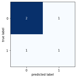
y_pred = id3.predict(data2, toyTree)
print('ID3 Decision Tree Classifier on ToyData dataset... \n')
print('-'*10 + 'Classification Report' + '-'*5)
print(metrics.classification_report(target2, y_pred))
print('-'*10 + 'Confusion Matrix' + '-'*10)
plot_confusion_matrix(metrics.confusion_matrix(target2, y_pred))
ID3 Decision Tree Classifier on ToyData dataset...

----------Classification Report-----
              precision    recall  f1-score   support

           +       0.67      0.67      0.67         3
           -       0.50      0.50      0.50         2

    accuracy                           0.60         5
   macro avg       0.58      0.58      0.58         5
weighted avg       0.60      0.60      0.60         5

----------Confusion Matrix----------
Testing ID3 with Scikit-learn digits
6. When you are sure that everything works properly, run the ID3-training for the digits training data you used in part 1. Do not constrain the training, i.e., run with default parameters. What do you see in the plot? Analyse the result (produce a confusion matrix and a classification report) and compare with the result from part 1 (when running with default parameters).
# Split digits data into training and test sets
X_train, X_test, y_train, y_test = train_test_split(digits.data, digits.target, test_size=0.3)
# Get attributes and classes for digits data
attributes = list(np.unique(X_train))
# Convert to tuple format for ID3 classifier
classes = tuple(np.unique(y_train))
# Initialise decision tree model
id3 = ID3DecisionTreeClassifier()
# Fit on digits training data (build tree)
digitsTree = id3.fit(X_train, y_train, attributes, classes, dataset="digits")
# Visualise tree with Graphviz
plot = id3.make_dot_data()
# Render tree in PDF
plot.render("myDigitsTree")
'myDigitsTree.pdf'
Due to the size of the tree, we’re unable to render it on a single PDF page. Run the code for yourself to visualise the results :-)
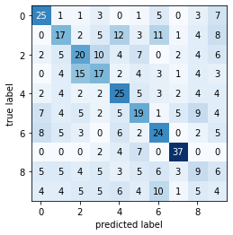
# Prediction over digits test data
y_pred = id3.predict(X_test, digitsTree, dataset="digits")
print('ID3 Decision Tree Classifier on Scikit-learn digits dataset... \n')
print('-'*10 + 'Classification Report' + '-'*5)
print(metrics.classification_report(y_test, y_pred))
print('-'*10 + 'Confusion Matrix' + '-'*10)
plot_confusion_matrix(metrics.confusion_matrix(y_test, y_pred))
ID3 Decision Tree Classifier on Scikit-learn digits dataset...

----------Classification Report-----
              precision    recall  f1-score   support

           0       0.33      0.30      0.32        53
           1       0.24      0.26      0.25        53
           2       0.30      0.29      0.29        49
           3       0.31      0.35      0.33        49
           4       0.37      0.31      0.34        61
           5       0.33      0.29      0.31        63
           6       0.31      0.50      0.38        38
           7       0.64      0.73      0.68        60
           8       0.13      0.12      0.12        58
           9       0.16      0.12      0.14        56

    accuracy                           0.32       540
   macro avg       0.31      0.33      0.32       540
weighted avg       0.32      0.32      0.32       540

----------Confusion Matrix----------
# Reshape data to 3D for visualisation
dim = int(np.sqrt(X_test.shape[1]))
X_test_images = X_test.reshape((len(X_test), dim, dim))
# Visualise random examples from digits dataset
visualize_random(X_test_images, y_test, examples_per_class=8)
# Convert predictions into numpy array
y_pred = np.array(y_pred)
# Visualise the images and their predicted labels
visualize_predictions(X_test_images, y_pred, examples_per_class=8)
Testing ID3 with modified (summarised) Scikit-learn digits
7. One striking difference should be in the ratio of breadth and depth of the two trees. Why is that the case? Modify your data set to contain only three values for the attributes (instead of potentially 16), e.g., ‘dark’, ‘grey’, and ‘light’, with for example ‘dark’ representing pixel values <5.0, and ‘light’ those >10.0. Train and test the classifier again. Do your results improve? Can you match the SKLearn implementation’s accuracy? If not, why do you think this is the case?
Bins:
Light: 0-4 –> 0Grey: 5-10 –> 1Dark: 11-16 –> 2
bin_bounds = [4, 10]
digits_data_summarised = np.digitize(digits.data, bins=bin_bounds, right=True)
digits_target_summarised = digits.target
X_train_bin, X_test_bin, y_train_bin, y_test_bin = train_test_split(digits_data_summarised, digits_target_summarised, test_size=0.3)
# Get attributes and classes for digits data
attributes_bin = list(np.unique(X_train_bin))
# Convert to tuple format for ID3 classifier
classes_bin = tuple(np.unique(y_train_bin))
# Initialise decision tree model
id3 = ID3DecisionTreeClassifier()
# Fit on digits summarised data (build tree)
digitsSummarisedTree = id3.fit(X_train_bin, y_train_bin, attributes_bin, classes_bin, dataset="digits_summarised")
# Visualise tree with Graphviz
plot = id3.make_dot_data()
# Render tree in PDF
plot.render("myDigitsSummarisedTree")
Due to the size of the tree, we’re unable to render it on a single PDF page. Run the code for yourself to visualise the results :-)
# Prediction over digits summarised test data
y_pred = id3.predict(X_test_bin, digitsSummarisedTree, dataset="digits_summarised")
print('ID3 Decision Tree Classifier on Scikit-learn digits (summarised) dataset... \n')
print('-'*10 + 'Classification Report' + '-'*5)
print(metrics.classification_report(y_test_bin, y_pred))
print('-'*10 + 'Confusion Matrix' + '-'*10)
plot_confusion_matrix(metrics.confusion_matrix(y_test_bin, y_pred))
ID3 Decision Tree Classifier on Scikit-learn digits (summarised) dataset...

----------Classification Report-----
              precision    recall  f1-score   support

           0       0.84      0.72      0.78        53
           1       0.61      0.70      0.65        56
           2       0.73      0.68      0.70        59
           3       0.64      0.69      0.66        51
           4       0.71      0.78      0.74        63
           5       0.69      0.72      0.71        50
           6       0.67      0.67      0.67        54
           7       0.88      0.86      0.87        49
           8       0.51      0.39      0.44        56
           9       0.56      0.63      0.60        49

    accuracy                           0.68       540
   macro avg       0.68      0.68      0.68       540
weighted avg       0.68      0.68      0.68       540

----------Confusion Matrix----------
# Reshape the test data to 3D for visualisation
dim = int(np.sqrt(X_test_bin.shape[1]))
X_test_bin_images = X_test_bin.reshape((len(X_test_bin),dim,dim))
# Visualise random images from digits summarised dataset
visualize_random(X_test_bin_images, y_test_bin, examples_per_class=8)
# Convert predictions into numpy array
y_pred = np.array(y_pred)
# Visualise the images and their predicted labels
visualize_predictions(X_test_bin_images, y_pred, examples_per_class=8)
8. (Bonus: If interested, explore the effects of different parameters regulating the depth of the tree, the maximum number of samples per leaf or required for a split, initially on the SKLearn version, but of course you can also implement them for your own classifier.) We’ll leave this exercise to the reader.
Congrats–you’ve reached the end of this article! By now, you should be familiar with decision trees for classification. You explored two popular decision tree algorithms: CART and ID3. You looked at the math behind the ID3 algorithm and wrote formulas to perform attribute selection using the information gain metric. You ran the CART and ID3 algorithms on data and measured their performance on multinomial classification. Lastly, you improved their results by (1) tweaking the hyperparameters and (2) modifying the data’s attribute values. While there is always more content to explore, we hope that this has been a fun and informative introduction for you.
Credits
This assignment was prepared by the EDAN95 HT2019 teaching staff at Lunds Tekniska Högskola (LTH). The skeleton code for the ID3-algorithm and ToyData dataset was authored by E.A. Topp (bio here).
Most of the code from the ID3 algorithm was inspired by A. Sears-Collins’ Iterative Dichotomiser 3 Algorithm in Python.
Additional credits:
-
GridSearchCVplotting method - sus_hml.
2019-11-15 00:00:00 -0800 - Written by Jonathan Logan Moran