CNN numpy keras image-augmentation feature-extraction transfer-learning classification flowers-recognition neural-networks machine-learning python ipynb Convolutional Neural Networks - The Basics
Jonathan L. Moran (jo6155mo-s@student.lu.se)
From the EDAN95 - Applied Machine Learning course given at Lunds Tekniska Högskola (LTH) | Ht2 2019.
In this post, we’ll introduce you to the Convolutional Neural Network and its application to image classification.
Objectives
In this assignment, we will
- Build a simple Convolutional Neural Network
- Use Image Augmentation
- Use a Pretrained Convolutional Base with and without image augmentation
Programming
Setting Up Google Colab
In case you aren’t already familiar with Google Colaboratory, head on over to https://colab.research.google.com and get started with your own cloud-hosted Jupyter notebook. There’s virtually no setup required and it’s free for our intended use. Google is kind enough to even throw in GPU access for free, which we will be using in the later part of this notebook. To get started, create a new notebook and upload our dataset by dragging the .zip file into the Files sidebar. The following steps will help you create a subdirectory and unzip the file.
### Load dataset into Google Colab
## 1. Create a folder in local directory
!mkdir src

## 2. Upload archive to Google Colab
# Drag and drop file from PC into Colab Files panel, then
# move the file into the 'src/' subdirectory

## 3. Unzip folder
!unzip src/archive.zip

# 4. Rename unzipped folder to 'flowers_original' and verify that the folder is in 'src' subdirectory
Collecting a dataset
For this image classification task, we will be using a popular multi-class classification dataset called the Flowers Recognition Kaggle dataset. This dataset consists of 4,242 low-resolution 2-D images each labeled with one of five flower types.
To follow along with this notebook, you should obtain a copy of the dataset via Kaggle at the link here.
### Splitting the dataset
# import flowers_create_dataset
"""
Categorising the flower dataset
Creating the dataset
Author: Pierre Nugues
"""
import os
from os import path
import random
import shutil

# The machine name (False if using Colab)
vilde = False

# To create the same dataset
random.seed(0)

# Here write the path to your dataset
if vilde:
    base = 'YOUR_LOCAL_DIRECTORY'
else:
    base = 'src/'
original_dataset_dir = os.path.join(base, 'flowers_original')
dataset = os.path.join(base, 'flowers_split')

train_dir = os.path.join(dataset, 'train')
validation_dir = os.path.join(dataset, 'validation')
test_dir = os.path.join(dataset, 'test')

categories = os.listdir(original_dataset_dir)
categories = [category for category in categories if not category.startswith('.')]
print('Image types:', categories)
data_folders = [os.path.join(original_dataset_dir, category) for category in categories]

pairs = []
for folder, category in zip(data_folders, categories):
    images = os.listdir(folder)
    images = [image for image in images if not image.startswith('.')]
    pairs.extend([(image, category) for image in images])

random.shuffle(pairs)
img_nbr = len(pairs)
train_images = pairs[0:int(0.6 * img_nbr)]
val_images = pairs[int(0.6 * img_nbr):int(0.8 * img_nbr)]
test_images = pairs[int(0.8 * img_nbr):]

# print(train_images)
print(len(train_images))
print(len(val_images))
print(len(test_images))

for image, label in train_images:
    src = os.path.join(original_dataset_dir, label, image)
    dst = os.path.join(train_dir, label, image)
    os.makedirs(os.path.dirname(dst), exist_ok=True)
    shutil.copyfile(src, dst)

for image, label in val_images:
    src = os.path.join(original_dataset_dir, label, image)
    dst = os.path.join(validation_dir, label, image)
    os.makedirs(os.path.dirname(dst), exist_ok=True)
    shutil.copyfile(src, dst)

for image, label in test_images:
    src = os.path.join(original_dataset_dir, label, image)
    dst = os.path.join(test_dir, label, image)
    os.makedirs(os.path.dirname(dst), exist_ok=True)
    shutil.copyfile(src, dst)
Image types: ['sunflower', 'tulip', 'rose', 'daisy', 'dandelion']
2590
863
864
The Flowers Recognition dataset consists of the following five class labels (flower types)
classes = ['daisy', 'dandelion', 'rose', 'sunflower', 'tulip']
def set_variables(base):
    base_dir = base
    train_dir = os.path.join(base_dir, 'train')
    validation_dir = os.path.join(base_dir, 'validation')
    test_dir = os.path.join(base_dir, 'test')
    return train_dir, validation_dir, test_dir
base_dir = 'src/flowers_split/'
train_dir, validation_dir, test_dir = set_variables(base_dir)
Now that we’ve collected our dataset and split it into train, test and validation sets, let’s move onto creating our first Convolutional Neural Network model.
Below is an outline of the first task and some suggestions from the EDAN95 course instructors
Building a Simple Convolutional Neural Network
- Create a simple convolutional network and train a model with the train set. You can start from the architecture proposed by Chollet, Listing 5.5 (in Chollet’s notebook 5.2), and a small number of epochs. Use the ImageDataGenerator class to scale your images as in the book: train_datagen = ImageDataGenerator(rescale=1. / 255) val_datagen = ImageDataGenerator(rescale=1. / 255) test_datagen = ImageDataGenerator(rescale=1. / 255)
- You will need to modify some parameters so that your network handles multiple classes.
- You will also adjust the number of steps so that your generator in the fitting procedure sees all the samples.
- You will report the training and validation losses and accuracies and comment on the possible overfit.
- Apply your network to the test set and report the accuracy as well as the confusion matrix you obtained. As with fitting, you may need to adjust the number of steps so that your network tests all the samples.
- Try to improve your model by modifying some parameters and evaluate your network again.
# Model parameters
epochs = 20
batch_size = 128
target_size = (150, 150)
Scaling our images
In order to prepare our data, the 2-D images, for use in our model, we have to first perform several pre-processing steps. This involves reading in our images in JPEG format, resizing them to 150x150px for faster processing, then converting their RGB pixel values into floating-point tensors. To help our neural network in the training process, we will also rescale pixel values from 0-255 to the same interval [0,1] for every image. This allows our images to contribute more evenly to the total loss (more on that here).
To accomplish this task in real-time, the Keras ImageDataGenerator class will be used.
# This is module with image preprocessing utilities
from keras.preprocessing import image
from keras.preprocessing.image import ImageDataGenerator
def data_preprocessing():
    # All images will be rescaled by 1./255
    train_datagen = ImageDataGenerator(rescale=1./255)
    test_datagen = ImageDataGenerator(rescale=1./255)

    train_generator = train_datagen.flow_from_directory(
        # This is the target directory
        train_dir,
        # All images will be resized to 150x150
        target_size=target_size,
        batch_size=batch_size,
        # Since we use categorical_crossentropy loss, we need categorical labels
        class_mode='categorical')

    validation_generator = test_datagen.flow_from_directory(
        validation_dir,
        target_size=target_size,
        batch_size=batch_size,
        class_mode='categorical')
    return train_datagen, test_datagen, train_generator, validation_generator
Let’s run our data generator and see how many images we have to process…
# Data preprocessing
train_datagen, test_datagen, train_generator, validation_generator = data_preprocessing()
Found 2590 images belonging to 5 classes.
Found 863 images belonging to 5 classes.
Checking to make sure we’ve specified the right image size in our generator…
print('image dimensions:', train_generator.target_size)
image dimensions: (150, 150)
Futhermore, we can take a look at the output of our train_generator to verify our image dimensions and the batch size (number of images per batch):
for data, labels in train_generator:
    print("data batch shape: (# samples={}, width(px)={}, height(px)={}, channels={})".format(data.shape[0], data.shape[1], data.shape[2], data.shape[3]))
    print("labels batch shape: (# samples={}, # classes={})".format(labels.shape[0], labels.shape[1]))
    break
data batch shape: (# samples=128, width(px)=150, height(px)=150, channels=3)
labels batch shape: (# samples=128, # classes=5)
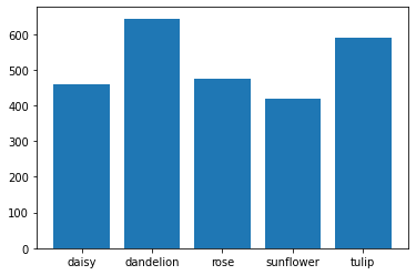
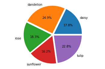
Visualising class representation
Since our dataset consists of five different classes (flower types), we want to first visualise the number of samples for each output class. To do so, we can get the count of the unique samples (images) in each class from our training set, then plot the counts on a bar chart using a familiar Python library.
from collections import OrderedDict
import numpy as np
unique, counts = np.unique(train_generator.classes, return_counts=True)
vals = OrderedDict(zip(unique, counts))

class_counts = []
for i in range(5):
  class_counts.append(vals[i])
import matplotlib.pyplot as plt
plt.figure()
x = np.arange(len(class_counts))
plt.bar(x, class_counts)
xlabel = list(train_generator.class_indices.keys())
plt.xticks(x, xlabel)
plt.show()
targets = [(counts)]
plt.pie(targets, labels=xlabel, explode=[0.05, 0.05, 0.05, 0.05, 0.05], autopct='%1.1f%%')
plt.axis('equal')
plt.show()
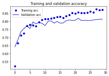
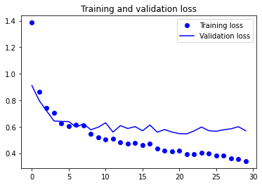
Visualising training performance
We’ll use the following plot_history() method to visualise our model’s training and validation accuracy and loss for each epoch. The input parameter is a History callback object which keeps track of the training metrics we want to visualise.
def plot_history(history):
    acc = history.history['categorical_accuracy']
    val_acc = history.history['val_categorical_accuracy']
    loss = history.history['loss']
    val_loss = history.history['val_loss']

    epochs = range(len(acc))

    plt.plot(epochs, acc, 'bo', label='Training acc')
    plt.plot(epochs, val_acc, 'b', label='Validation acc')
    plt.title('Training and validation accuracy')
    plt.legend()

    plt.figure()
    plt.plot(epochs, loss, 'bo', label='Training loss')
    plt.plot(epochs, val_loss, 'b', label='Validation loss')
    plt.title('Training and validation loss')
    plt.legend()

    plt.show()
Building the network
The structure of our Convolutional Neural Network (CNN) is defined as a Keras Sequential model with a stack of alternating Conv2D and MaxPooling2D layers. At the core of our CNN is the Conv2D layer which transforms the input and outputs the transformation to the next layer. The tranformation performed in Conv2D is known as a convolution operation. In this operation, a filter is applied over the entire input in a sliding window protocol (from top-left to bottom-right of the matrix). The dot product is computed at each step and its resulting value is stored in the output channel. Once the filter has convolved the entire input, a new representation of our input is formed. This output channel is referred to as a feature map. Most commonly, a filter is applied over an input image to detect patterns such as edges, curves or textures. For a more complete understanding of the convolutional layer, read this article.
The MaxPooling2D layer combination is used to reduce the dimensionality of the input (image) by reducing the number of pixels in the output from the previous convolutional layer. This reduces the amount of computation performed and the number of parameters to learn from the feature map.
To speed up our model training, we will use the ReLU (Rectified Linear Unit) activation function in our Conv2D layers. This function returns 0 if it receives any negative input, otherwise it will return the positve input value x. This function speeds up the gradient computation by setting any negative values to zero. For futher reading, see this article about ReLU on Keras.
from keras import layers
from keras import models
from keras import optimizers
from keras import metrics
from tensorflow.keras.utils import to_categorical
# Building our network (Conv2D/MaxPooling2D stack + Dense/Flatten layer)
def build_network():
    model = models.Sequential()
    model.add(layers.Conv2D(filters=32, kernel_size=(3, 3), activation='relu', input_shape=(150,150,3)))
    model.add(layers.MaxPooling2D(pool_size=(2, 2)))
    model.add(layers.Conv2D(filters=64, kernel_size=(3, 3), activation='relu'))
    model.add(layers.MaxPooling2D(pool_size=(2, 2)))
    model.add(layers.Conv2D(filters=128, kernel_size=(3, 3), activation='relu'))
    model.add(layers.MaxPooling2D(pool_size=(2, 2)))
    model.add(layers.Conv2D(filters=128, kernel_size=(3, 3), activation='relu'))
    model.add(layers.MaxPooling2D(pool_size=(2, 2)))
    # This converts our 3-D feature maps into 1-D feature vectors
    model.add(layers.Flatten())
    model.add(layers.Dense(512, activation='relu'))
    model.add(layers.Dense(len(classes), activation='softmax'))

    print(model.summary())

    model.compile(loss='categorical_crossentropy',
                  optimizer=optimizers.RMSprop(),
                  metrics =['categorical_accuracy'])

    return model
model = build_network()
Model: "sequential"
_________________________________________________________________
Layer (type)                 Output Shape              Param #
=================================================================
conv2d (Conv2D)              (None, 148, 148, 32)      896
_________________________________________________________________
max_pooling2d (MaxPooling2D) (None, 74, 74, 32)        0
_________________________________________________________________
conv2d_1 (Conv2D)            (None, 72, 72, 64)        18496
_________________________________________________________________
max_pooling2d_1 (MaxPooling2 (None, 36, 36, 64)        0
_________________________________________________________________
conv2d_2 (Conv2D)            (None, 34, 34, 128)       73856
_________________________________________________________________
max_pooling2d_2 (MaxPooling2 (None, 17, 17, 128)       0
_________________________________________________________________
conv2d_3 (Conv2D)            (None, 15, 15, 128)       147584
_________________________________________________________________
max_pooling2d_3 (MaxPooling2 (None, 7, 7, 128)         0
_________________________________________________________________
flatten (Flatten)            (None, 6272)              0
_________________________________________________________________
dense (Dense)                (None, 512)               3211776
_________________________________________________________________
dense_1 (Dense)              (None, 5)                 2565
=================================================================
Total params: 3,455,173
Trainable params: 3,455,173
Non-trainable params: 0
_________________________________________________________________
None
From the above model summary, we can see two things. One is that our feature map size decreases from 150x150 in our first Conv2D layer to 15x15 in our last Conv2D layer. Another is that the feature map depth increases from 32 to 128 as the network progresses. François Chollet–the creator of Keras, notes that this is a common pattern in almost all convnets.
The last layer in our model is specific to our task of multi-class classification. We expect a final layer of size 5, where each node corresponds to one of the five total classes (flower types). A softmax last-layer activation function is used to predict a multinomial probability distribution, or, in other words, the likelihood each image corresponds to one of the five possible target classes. The softmax constraint specifies that the sum of the five probability values must add up to 1.0. After our prediction, we will use the argmax function to “select” the most-likely class label (one with the greatest probability value) for each predicted sample in our output.
Training the model
Now that we’ve built our first CNN, it’s time to run it through our training data. In order to do that, we use the keras.preprocessing.image ImageDataGenerator class we specified earlier. The fit_generator method takes all the same parameters as a standard fit method aside from the first and most important one–the input train_generator object. This object “batches” our training data into pre-processed chunks, performing the resizing and normalising of our images according to the specifications we set at the start of this notebook. To be more precise about our other parameters, we must remember which batch_size we set for our train_generator. In our case, this was set to 128. This means that 128 images will be fetched from our training set directory, pre-processed, then fed into our network. During each epoch, we pass through every example in our training set. Thus, we must also specify the number of steps_per_epoch such that every training example is seen in each epoch for n number of batches. The following np.ceil calculation helps you in determining that amount.
def train_model(model, epochs=1):
    history = model.fit_generator(
        train_generator,
        steps_per_epoch=np.ceil(train_generator.samples / train_generator.batch_size),
        epochs=epochs,
        validation_data=validation_generator,
        validation_steps=np.ceil(validation_generator.samples / validation_generator.batch_size))

    plot_history(history)
train_model(model, epochs)
/usr/local/lib/python3.7/dist-packages/keras/engine/training.py:1915: UserWarning: `Model.fit_generator` is deprecated and will be removed in a future version. Please use `Model.fit`, which supports generators.
  warnings.warn('`Model.fit_generator` is deprecated and '


Epoch 1/20
21/21 [==============================] - 55s 497ms/step - loss: 2.2696 - categorical_accuracy: 0.2717 - val_loss: 1.3862 - val_categorical_accuracy: 0.3893
Epoch 2/20
21/21 [==============================] - 9s 424ms/step - loss: 1.3096 - categorical_accuracy: 0.4251 - val_loss: 1.2477 - val_categorical_accuracy: 0.5087
Epoch 3/20
21/21 [==============================] - 9s 423ms/step - loss: 1.2210 - categorical_accuracy: 0.4956 - val_loss: 1.1674 - val_categorical_accuracy: 0.5377
Epoch 4/20
21/21 [==============================] - 9s 416ms/step - loss: 1.1635 - categorical_accuracy: 0.5424 - val_loss: 1.0487 - val_categorical_accuracy: 0.5944
Epoch 5/20
21/21 [==============================] - 9s 423ms/step - loss: 1.0198 - categorical_accuracy: 0.5894 - val_loss: 1.0173 - val_categorical_accuracy: 0.5840
Epoch 6/20
21/21 [==============================] - 9s 432ms/step - loss: 0.9581 - categorical_accuracy: 0.6158 - val_loss: 0.9551 - val_categorical_accuracy: 0.6165
Epoch 7/20
21/21 [==============================] - 9s 421ms/step - loss: 0.9083 - categorical_accuracy: 0.6492 - val_loss: 1.1493 - val_categorical_accuracy: 0.5446
Epoch 8/20
21/21 [==============================] - 9s 422ms/step - loss: 0.8449 - categorical_accuracy: 0.6799 - val_loss: 0.9085 - val_categorical_accuracy: 0.6466
Epoch 9/20
21/21 [==============================] - 9s 427ms/step - loss: 0.6936 - categorical_accuracy: 0.7421 - val_loss: 0.8759 - val_categorical_accuracy: 0.6570
Epoch 10/20
21/21 [==============================] - 9s 426ms/step - loss: 0.6667 - categorical_accuracy: 0.7407 - val_loss: 0.9266 - val_categorical_accuracy: 0.6385
Epoch 11/20
21/21 [==============================] - 9s 425ms/step - loss: 0.6070 - categorical_accuracy: 0.7652 - val_loss: 0.9943 - val_categorical_accuracy: 0.6593
Epoch 12/20
21/21 [==============================] - 9s 420ms/step - loss: 0.5550 - categorical_accuracy: 0.7833 - val_loss: 1.2728 - val_categorical_accuracy: 0.5585
Epoch 13/20
21/21 [==============================] - 9s 423ms/step - loss: 0.4671 - categorical_accuracy: 0.8275 - val_loss: 1.2127 - val_categorical_accuracy: 0.5736
Epoch 14/20
21/21 [==============================] - 9s 418ms/step - loss: 0.4220 - categorical_accuracy: 0.8507 - val_loss: 1.0448 - val_categorical_accuracy: 0.6419
Epoch 15/20
21/21 [==============================] - 9s 415ms/step - loss: 0.2842 - categorical_accuracy: 0.9049 - val_loss: 1.3287 - val_categorical_accuracy: 0.6130
Epoch 16/20
21/21 [==============================] - 9s 418ms/step - loss: 0.3114 - categorical_accuracy: 0.8970 - val_loss: 1.4184 - val_categorical_accuracy: 0.6373
Epoch 17/20
21/21 [==============================] - 9s 423ms/step - loss: 0.1621 - categorical_accuracy: 0.9489 - val_loss: 1.3792 - val_categorical_accuracy: 0.6605
Epoch 18/20
21/21 [==============================] - 9s 423ms/step - loss: 0.2085 - categorical_accuracy: 0.9573 - val_loss: 1.3858 - val_categorical_accuracy: 0.6535
Epoch 19/20
21/21 [==============================] - 9s 421ms/step - loss: 0.0811 - categorical_accuracy: 0.9847 - val_loss: 1.2699 - val_categorical_accuracy: 0.6280
Epoch 20/20
21/21 [==============================] - 9s 421ms/step - loss: 0.0848 - categorical_accuracy: 0.9850 - val_loss: 2.1311 - val_categorical_accuracy: 0.6176

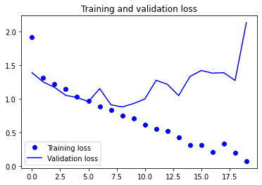
For a simple Convolutional Neural Network, our initial results don’t look all that bad! However, examining the plots a bit closer we see that the validation accuracy reaches a maximum around the 10th epoch. We also see that our validation loss reaches a minimum around the 7th epoch. Conversely, our training loss appears to decrease linearly until it reaches 0. This is characteristic of overfitting.
Why does this behavior occur? Well, a simple answer is that the number of training samples we have (ca. 2000) is relatively few. In order to combat overfitting, there are many popular techniques from adding Dropout layers to penalising our model’s weights with weight decay (L2 regularisation). Another technique specific to computer vision is data augmentation. We’ll be using this in our next model to improve our results.
Evaluating model performance
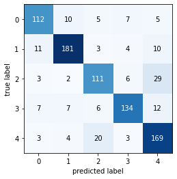
For the ML enthusiasts out there, we’ll report our model’s performance on several important metrics, namely precision, recall, and f1-score. In addition to generating a classification report, we’ll produce a confusion matrix to quantify how many misclassifications our model is making.
from sklearn.metrics import confusion_matrix, classification_report
from mlxtend.plotting import plot_confusion_matrix
def evaluate_model(model):
    test_generator = test_datagen.flow_from_directory(
        test_dir,
        target_size=target_size,
        batch_size=batch_size,
        class_mode='categorical',
        shuffle=False)

    y_prob = model.predict_generator(test_generator, np.ceil(test_generator.samples / test_generator.batch_size))
    # Select greatest class probability for each sample in y_prob
    y_pred = np.argmax(y_prob, axis=1)

    print('-'*10 + 'Classification Report' + '-'*5)
    print(classification_report(test_generator.classes, y_pred, target_names=classes))
    print('-'*10 + 'Confusion Matrix' + '-'*10)
    #print(confusion_matrix(test_generator.classes, y_pred))
    plot_confusion_matrix(confusion_matrix(test_generator.classes, y_pred))
y_pred = evaluate_model(model)
Found 864 images belonging to 5 classes.

----------Classification Report-----
              precision    recall  f1-score   support

       daisy       0.63      0.60      0.62       139
   dandelion       0.68      0.80      0.74       209
        rose       0.73      0.22      0.34       151
   sunflower       0.71      0.75      0.73       166
       tulip       0.58      0.77      0.66       199

    accuracy                           0.65       864
   macro avg       0.67      0.63      0.62       864
weighted avg       0.66      0.65      0.63       864

----------Confusion Matrix----------
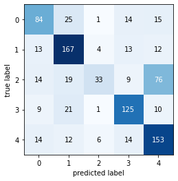
So, our model’s overall F1 score was 0.65 or ca. 65% accuracy. We’ll use this as a benchmark to compare to as we make incremental progress in the following models.
In the next model, we’ll be using a clever approach to tackle overfitting specific to deep learning models for computer vision applications. This approach involves generating new data (more images) by “augmenting” the existing samples. We accomplish this by applying a number of random transformations to the images in our dataset to produce more samples that appear new to the model. Our handy Keras ImageDataGenerator allows us to do just that while remaining consistent with our batched, pre-processed image pipeline.
Here’s an outline of what we will accomplish…
Using Image Augmentation
- The flower dataset is relatively small. A way to expand such datasets is to generate artificial images by applying small transformations to existing images. Keras provides a built-in class for this: ImageDataGenerator. You will reuse it and apply it to the flower data set.
- Using the network from the previous exercise, apply some transformations to your images. You can start from Chollet, Listing 5.11 (in notebook 5.2 also).
- Report the training and validation losses and accuracies and comment on the possible overfit.
- Apply your network to the test set and report the accuracy as well as the confusion matrix you obtained.
# The data augmentation generator
datagen = ImageDataGenerator(
    rescale=1./255,
    rotation_range=40,
    width_shift_range=0.2,
    height_shift_range=0.2,
    shear_range=0.2,
    zoom_range=0.2,
    horizontal_flip=True,
    fill_mode='nearest')
In order to better understand each of the parameters in our datagen, here’s a description provided to us by F. Chollet:
rotation_rangeis a value in degrees (0-180), a range within which to randomly rotate pictures.width_shiftand height_shift are ranges (as a fraction of total width or height) within which to randomly translate pictures vertically or horizontally.shear_rangeis for randomly applying shearing transformations.zoom_rangeis for randomly zooming inside pictures.horizontal_flipis for randomly flipping half of the images horizontally – relevant when there are no assumptions of horizontal asymmetry (e.g. real-world pictures).fill_modeis the strategy used for filling in newly created pixels, which can appear after a rotation or a width/height shift.
Visualising the augmented images
With our datagen parameters specified, we have successfully completed the first step in our augmentation process.
Let’s visualise a set of our augmented images…
from keras.preprocessing import image
# Selecting the "daisy" class images from the training set
folder_path = 'src/flowers_split/train/daisy'

file_names = [os.path.join(folder_path, fname) for fname in os.listdir(folder_path)]

# We pick one image to "augment"
img_path = file_names[50]

# Read the image and resize it
img = image.load_img(img_path, target_size=target_size)

# Convert it to a Numpy array with shape (150, 150, 3)
x = image.img_to_array(img)

# Reshape it to (1, 150, 150, 3)
x = x.reshape((1,) + x.shape)

# The .flow() command below generates batches of randomly transformed images.
# It will loop indefinitely, so we need to `break` the loop at some point!
i = 0
for batch in datagen.flow(x, batch_size=1):
    plt.figure(i)
    imgplot = plt.imshow(image.array_to_img(batch[0]))
    i += 1
    if i % 4 == 0:
        break

plt.show()
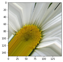
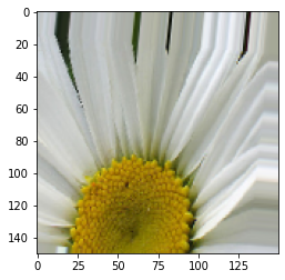
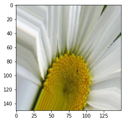
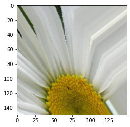
Great! We’ll now be able to train our model on a larger dataset using more images like the samples above. However, there’s still one extra step we must take to prevent overfitting. The input images, although augmented, are still heavily intercorrelated with the original dataset. In other words, most of the “new” information we’ve introduced is from our original data. To help address this issue, we add a Dropout layer to our model.
Training our model using data augmentation and dropout
To further fight overfitting, we will also add a Dropout layer to our model, right before the densely-connected classifier. Dropout is a regularization technique that helps prevent the model from overfitting by randomly “dropping” nuerons from the network in each training iteration. The goal of dropout is to encourage each hidden unit in the neural network to “learn” to work with a random set of surviving hidden units (neurons), creating a more robust network. This happens because each hidden unit must learn to encode a representation of the feature map without relying on other hidden units that might be “dropped” over the training iterations.
# Building our network (Conv2D/MaxPooling2D stack + Dropout + Dense/Flatten layer)
def build_network():
    model = models.Sequential()
    model.add(layers.Conv2D(filters=32, kernel_size=(3, 3), activation='relu', input_shape=(150,150,3)))
    model.add(layers.MaxPooling2D(pool_size=(2, 2)))
    model.add(layers.Conv2D(filters=64, kernel_size=(3, 3), activation='relu'))
    model.add(layers.MaxPooling2D(pool_size=(2, 2)))
    model.add(layers.Conv2D(filters=128, kernel_size=(3, 3), activation='relu'))
    model.add(layers.MaxPooling2D(pool_size=(2, 2)))
    model.add(layers.Conv2D(filters=128, kernel_size=(3, 3), activation='relu'))
    model.add(layers.MaxPooling2D(pool_size=(2, 2)))
    # This converts our 3-D feature maps into 1-D feature vectors
    model.add(layers.Flatten())
    # Here we set our dropout rate to 0.2
    model.add(layers.Dropout(0.2))
    model.add(layers.Dense(512, activation='relu'))
    model.add(layers.Dense(5, activation='softmax'))

    print(model.summary())
    # Setting learning rate manually
    model.compile(loss='categorical_crossentropy',
                  optimizer=optimizers.RMSprop(learning_rate=1e-5),
                  #optimizer=optimizers.Adam(learning_rate=1e-4),
                  metrics =['categorical_accuracy'])

    return model
model = build_network()
Model: "sequential_1"
_________________________________________________________________
Layer (type)                 Output Shape              Param #
=================================================================
conv2d_4 (Conv2D)            (None, 148, 148, 32)      896
_________________________________________________________________
max_pooling2d_4 (MaxPooling2 (None, 74, 74, 32)        0
_________________________________________________________________
conv2d_5 (Conv2D)            (None, 72, 72, 64)        18496
_________________________________________________________________
max_pooling2d_5 (MaxPooling2 (None, 36, 36, 64)        0
_________________________________________________________________
conv2d_6 (Conv2D)            (None, 34, 34, 128)       73856
_________________________________________________________________
max_pooling2d_6 (MaxPooling2 (None, 17, 17, 128)       0
_________________________________________________________________
conv2d_7 (Conv2D)            (None, 15, 15, 128)       147584
_________________________________________________________________
max_pooling2d_7 (MaxPooling2 (None, 7, 7, 128)         0
_________________________________________________________________
flatten_1 (Flatten)          (None, 6272)              0
_________________________________________________________________
dropout (Dropout)            (None, 6272)              0
_________________________________________________________________
dense_2 (Dense)              (None, 512)               3211776
_________________________________________________________________
dense_3 (Dense)              (None, 5)                 2565
=================================================================
Total params: 3,455,173
Trainable params: 3,455,173
Non-trainable params: 0
_________________________________________________________________
None
Training the model
We’ll now train our updated model on the augmented images and visualise our training performance. Since we want to increase the number of samples seen by our model, we will train our model for 100 epochs (up from 20). This will allow our datagen to generate more augmented samples than previously seen in the original, unmodified set.
import time
def train_model(model, epochs=100):
    start_time = time.time()
    train_datagen = ImageDataGenerator(
        rescale=1./255,
        rotation_range=40,
        width_shift_range=0.2,
        height_shift_range=0.2,
        shear_range=0.2,
        zoom_range=0.2,
        horizontal_flip=True,
        fill_mode='nearest')

    test_datagen = ImageDataGenerator(rescale=1./255)

    train_generator = train_datagen.flow_from_directory(
        # This is the target directory
        train_dir,
        # All images will be resized to 150x150
        target_size=target_size,
        batch_size=batch_size,
        class_mode='categorical')

    # Note that validation data shouldn't be augmented
    validation_generator = test_datagen.flow_from_directory(
        validation_dir,
        target_size=(150, 150),
        batch_size=batch_size,
        class_mode='categorical')

    history = model.fit_generator(
        train_generator,
        steps_per_epoch=np.ceil(train_generator.samples / train_generator.batch_size),
        epochs=epochs,
        validation_data=validation_generator,
        validation_steps=np.ceil(validation_generator.samples / validation_generator.batch_size))

    print('Total training time (sec):', time.time() - start_time)
    plot_history(history)
train_model(model, epochs=100)
Found 2590 images belonging to 5 classes.
Found 863 images belonging to 5 classes.


Epoch 1/100
21/21 [==============================] - 21s 942ms/step - loss: 1.6016 - categorical_accuracy: 0.2513 - val_loss: 1.5848 - val_categorical_accuracy: 0.2607
Epoch 2/100
21/21 [==============================] - 19s 909ms/step - loss: 1.5827 - categorical_accuracy: 0.3129 - val_loss: 1.5675 - val_categorical_accuracy: 0.2885
Epoch 3/100
21/21 [==============================] - 19s 916ms/step - loss: 1.5657 - categorical_accuracy: 0.3126 - val_loss: 1.5458 - val_categorical_accuracy: 0.3071
Epoch 4/100
21/21 [==============================] - 19s 912ms/step - loss: 1.5416 - categorical_accuracy: 0.3368 - val_loss: 1.5163 - val_categorical_accuracy: 0.3407
Epoch 5/100
21/21 [==============================] - 19s 912ms/step - loss: 1.5142 - categorical_accuracy: 0.3656 - val_loss: 1.4830 - val_categorical_accuracy: 0.3859
Epoch 6/100
21/21 [==============================] - 19s 909ms/step - loss: 1.4887 - categorical_accuracy: 0.3912 - val_loss: 1.4488 - val_categorical_accuracy: 0.4148
Epoch 7/100
21/21 [==============================] - 19s 916ms/step - loss: 1.4581 - categorical_accuracy: 0.4016 - val_loss: 1.4160 - val_categorical_accuracy: 0.4299
Epoch 8/100
21/21 [==============================] - 19s 911ms/step - loss: 1.4225 - categorical_accuracy: 0.4081 - val_loss: 1.3844 - val_categorical_accuracy: 0.4264
Epoch 9/100
21/21 [==============================] - 19s 913ms/step - loss: 1.3931 - categorical_accuracy: 0.4142 - val_loss: 1.3523 - val_categorical_accuracy: 0.4403
Epoch 10/100
21/21 [==============================] - 19s 914ms/step - loss: 1.3612 - categorical_accuracy: 0.4365 - val_loss: 1.3337 - val_categorical_accuracy: 0.4299
...
Epoch 90/100
21/21 [==============================] - 19s 905ms/step - loss: 1.0141 - categorical_accuracy: 0.6017 - val_loss: 1.0311 - val_categorical_accuracy: 0.5921
Epoch 91/100
21/21 [==============================] - 19s 916ms/step - loss: 1.0187 - categorical_accuracy: 0.5853 - val_loss: 1.0427 - val_categorical_accuracy: 0.6025
Epoch 92/100
21/21 [==============================] - 19s 910ms/step - loss: 0.9943 - categorical_accuracy: 0.6174 - val_loss: 1.0525 - val_categorical_accuracy: 0.5910
Epoch 93/100
21/21 [==============================] - 19s 915ms/step - loss: 1.0183 - categorical_accuracy: 0.6032 - val_loss: 1.0369 - val_categorical_accuracy: 0.5933
Epoch 94/100
21/21 [==============================] - 19s 912ms/step - loss: 1.0044 - categorical_accuracy: 0.5981 - val_loss: 1.0369 - val_categorical_accuracy: 0.6002
Epoch 95/100
21/21 [==============================] - 19s 909ms/step - loss: 1.0113 - categorical_accuracy: 0.5913 - val_loss: 1.0419 - val_categorical_accuracy: 0.6014
Epoch 96/100
21/21 [==============================] - 19s 950ms/step - loss: 1.0083 - categorical_accuracy: 0.6036 - val_loss: 1.0568 - val_categorical_accuracy: 0.6014
Epoch 97/100
21/21 [==============================] - 19s 914ms/step - loss: 0.9845 - categorical_accuracy: 0.6243 - val_loss: 1.0390 - val_categorical_accuracy: 0.6002
Epoch 98/100
21/21 [==============================] - 19s 914ms/step - loss: 1.0517 - categorical_accuracy: 0.5830 - val_loss: 1.0564 - val_categorical_accuracy: 0.6025
Epoch 99/100
21/21 [==============================] - 19s 909ms/step - loss: 1.0178 - categorical_accuracy: 0.6036 - val_loss: 1.0428 - val_categorical_accuracy: 0.5979
Epoch 100/100
21/21 [==============================] - 19s 912ms/step - loss: 1.0076 - categorical_accuracy: 0.5935 - val_loss: 1.0857 - val_categorical_accuracy: 0.5921
Total training time (sec): 1925.0976030826569

Evaluating model performance
def evaluate_model(model):
    test_generator = test_datagen.flow_from_directory(
        test_dir,
        shuffle=False,
        target_size=target_size,
        batch_size=batch_size,
        class_mode='categorical')

    y_prob = model.predict_generator(test_generator,
                                     np.ceil(test_generator.samples / test_generator.batch_size))
    # Select class label with highest probability
    y_pred = np.argmax(y_prob, axis=1)

    print('-'*10 + 'Classification Report' + '-'*5)
    print(classification_report(test_generator.classes, y_pred, target_names=classes))
    print('-'*10 + 'Confusion Matrix' + '-'*10)
    plot_confusion_matrix(confusion_matrix(test_generator.classes, y_pred))
evaluate_model(model)
Found 864 images belonging to 5 classes.


----------Classification Report-----
              precision    recall  f1-score   support

       daisy       0.63      0.58      0.60       139
   dandelion       0.73      0.61      0.67       209
        rose       0.66      0.44      0.53       151
   sunflower       0.53      0.88      0.66       166
       tulip       0.64      0.59      0.61       199

    accuracy                           0.62       864
   macro avg       0.64      0.62      0.61       864
weighted avg       0.64      0.62      0.62       864

----------Confusion Matrix----------
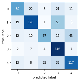
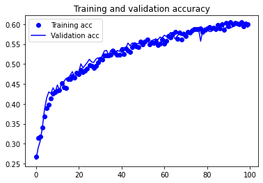
While the augmented images didn’t seem to improve the model’s F1 score, our model’s training curves indicate that we are no longer overfitting. In other words, our training curve more closely matches the validation curve. In the next section of this notebook, we will be improving the accuracy of our classifier with a pre-trained model via a technique called transfer learning.
Using a Pretrained Convolutional Base
A common and highly effective approach to deep learning on small image datasets is to use a pretrained network. A pretrained network is a saved network that was previously trained on a large dataset, typically on a large-scale image-classification task. (F. Chollet, Ch. 5.3 - Deep Learning with Python). What makes the use of pretrained convolutional bases desirable is that these networks are often trained on large enough datasets (e.g. ImageNet’s 1.4 mil. labeled images of 1,000 classes) that the pretrained network’s learned representations can encompass a general enough model of the visual world. Through feature extraction and fine-tuning techniques, we can “port” the learned features of the pretrained convbases across other models, such as our own. In the next section of this notebook, we’ll be exploring the InceptionV3 pretrained convolutional base and applying it to our own model using a feature extraction approach.
Feature extraction without data augmentation
- Build a network that consists of the Inception V3 convolutional base and two dense layers. As in Chollet, Listing 5.17 (in Chollet’s notebook 5.3), you will program an
extract_features()function. - Train your network and report the training and validation losses and accuracies.
- Apply your network to the test set and report the accuracy as well as the confusion matrix you obtained.
# Model parameters
epochs = 20
batch_size = 128
target_size = (150, 150)
Our first step is to select a pretrained network. For this task, we will use Google’s InceptionV3. This is a Keras image classification model that has been optionally loaded with weights pre-trained on the ImageNet dataset. The InceptionV3 is referred to as our “convolutional base”. Note that the densely-connected classifier of the InceptionV3 has been removed (with parameter include_top=False). The reason for this decision is that our pretrained network’s output, the densely-connected prediction layer, is not usable for our task specific to classifying a subset of five flower types. The ImageNet dataset used to train the InceptionV3 consists of 1,000 unique classes, and thus we will not have any use for the majority of the model’s output tensors (the distinct classes’ probability distributions).
Thankfully, Keras provides us with a simple way to leave this part of the model out. Instead, we will be preserving layers that come earlier in the InceptionV3 which extract local, highly generic feature maps (such as visual edges, colors, and textures).
# Importing the pretrained network as a Keras model
from tensorflow.keras.applications import InceptionV3
# Initialising our conv_base object with desired parameters
conv_base = InceptionV3(weights='imagenet',
                        include_top=False,
                        input_shape=(150, 150, 3))
Downloading data from https://storage.googleapis.com/tensorflow/keras-applications/inception_v3/inception_v3_weights_tf_dim_ordering_tf_kernels_notop.h5
87916544/87910968 [==============================] - 0s 0us/step
Let’s look at the architecture of our convolutional base in detail…
conv_base.summary()
Model: "inception_v3"
__________________________________________________________________________________________________
Layer (type)                    Output Shape         Param #     Connected to
==================================================================================================
input_1 (InputLayer)            [(None, 150, 150, 3) 0
__________________________________________________________________________________________________
conv2d (Conv2D)                 (None, 74, 74, 32)   864         input_1[0][0]
__________________________________________________________________________________________________
batch_normalization (BatchNorma (None, 74, 74, 32)   96          conv2d[0][0]
__________________________________________________________________________________________________
activation (Activation)         (None, 74, 74, 32)   0           batch_normalization[0][0]
__________________________________________________________________________________________________
conv2d_1 (Conv2D)               (None, 72, 72, 32)   9216        activation[0][0]
__________________________________________________________________________________________________
batch_normalization_1 (BatchNor (None, 72, 72, 32)   96          conv2d_1[0][0]
__________________________________________________________________________________________________
activation_1 (Activation)       (None, 72, 72, 32)   0           batch_normalization_1[0][0]
__________________________________________________________________________________________________
conv2d_2 (Conv2D)               (None, 72, 72, 64)   18432       activation_1[0][0]
__________________________________________________________________________________________________
batch_normalization_2 (BatchNor (None, 72, 72, 64)   192         conv2d_2[0][0]
__________________________________________________________________________________________________
activation_2 (Activation)       (None, 72, 72, 64)   0           batch_normalization_2[0][0]
__________________________________________________________________________________________________
max_pooling2d (MaxPooling2D)    (None, 35, 35, 64)   0           activation_2[0][0]
__________________________________________________________________________________________________
conv2d_3 (Conv2D)               (None, 35, 35, 80)   5120        max_pooling2d[0][0]
__________________________________________________________________________________________________
batch_normalization_3 (BatchNor (None, 35, 35, 80)   240         conv2d_3[0][0]
__________________________________________________________________________________________________
activation_3 (Activation)       (None, 35, 35, 80)   0           batch_normalization_3[0][0]
__________________________________________________________________________________________________
conv2d_4 (Conv2D)               (None, 33, 33, 192)  138240      activation_3[0][0]
__________________________________________________________________________________________________
batch_normalization_4 (BatchNor (None, 33, 33, 192)  576         conv2d_4[0][0]
__________________________________________________________________________________________________
activation_4 (Activation)       (None, 33, 33, 192)  0           batch_normalization_4[0][0]
__________________________________________________________________________________________________
max_pooling2d_1 (MaxPooling2D)  (None, 16, 16, 192)  0           activation_4[0][0]
__________________________________________________________________________________________________
conv2d_8 (Conv2D)               (None, 16, 16, 64)   12288       max_pooling2d_1[0][0]
__________________________________________________________________________________________________
batch_normalization_8 (BatchNor (None, 16, 16, 64)   192         conv2d_8[0][0]
__________________________________________________________________________________________________
activation_8 (Activation)       (None, 16, 16, 64)   0           batch_normalization_8[0][0]
__________________________________________________________________________________________________
conv2d_6 (Conv2D)               (None, 16, 16, 48)   9216        max_pooling2d_1[0][0]
__________________________________________________________________________________________________
conv2d_9 (Conv2D)               (None, 16, 16, 96)   55296       activation_8[0][0]
__________________________________________________________________________________________________
batch_normalization_6 (BatchNor (None, 16, 16, 48)   144         conv2d_6[0][0]
__________________________________________________________________________________________________
batch_normalization_9 (BatchNor (None, 16, 16, 96)   288         conv2d_9[0][0]
__________________________________________________________________________________________________
activation_6 (Activation)       (None, 16, 16, 48)   0           batch_normalization_6[0][0]
__________________________________________________________________________________________________
activation_9 (Activation)       (None, 16, 16, 96)   0           batch_normalization_9[0][0]
__________________________________________________________________________________________________
average_pooling2d (AveragePooli (None, 16, 16, 192)  0           max_pooling2d_1[0][0]
__________________________________________________________________________________________________
conv2d_5 (Conv2D)               (None, 16, 16, 64)   12288       max_pooling2d_1[0][0]
__________________________________________________________________________________________________
conv2d_7 (Conv2D)               (None, 16, 16, 64)   76800       activation_6[0][0]
__________________________________________________________________________________________________
conv2d_10 (Conv2D)              (None, 16, 16, 96)   82944       activation_9[0][0]
__________________________________________________________________________________________________
conv2d_11 (Conv2D)              (None, 16, 16, 32)   6144        average_pooling2d[0][0]
__________________________________________________________________________________________________
batch_normalization_5 (BatchNor (None, 16, 16, 64)   192         conv2d_5[0][0]
__________________________________________________________________________________________________
batch_normalization_7 (BatchNor (None, 16, 16, 64)   192         conv2d_7[0][0]
__________________________________________________________________________________________________
batch_normalization_10 (BatchNo (None, 16, 16, 96)   288         conv2d_10[0][0]
__________________________________________________________________________________________________
batch_normalization_11 (BatchNo (None, 16, 16, 32)   96          conv2d_11[0][0]
__________________________________________________________________________________________________
activation_5 (Activation)       (None, 16, 16, 64)   0           batch_normalization_5[0][0]
__________________________________________________________________________________________________
activation_7 (Activation)       (None, 16, 16, 64)   0           batch_normalization_7[0][0]
__________________________________________________________________________________________________
activation_10 (Activation)      (None, 16, 16, 96)   0           batch_normalization_10[0][0]
__________________________________________________________________________________________________
activation_11 (Activation)      (None, 16, 16, 32)   0           batch_normalization_11[0][0]
__________________________________________________________________________________________________
mixed0 (Concatenate)            (None, 16, 16, 256)  0           activation_5[0][0]
                                                                 activation_7[0][0]
                                                                 activation_10[0][0]
                                                                 activation_11[0][0]
__________________________________________________________________________________________________
conv2d_15 (Conv2D)              (None, 16, 16, 64)   16384       mixed0[0][0]
__________________________________________________________________________________________________
batch_normalization_15 (BatchNo (None, 16, 16, 64)   192         conv2d_15[0][0]
__________________________________________________________________________________________________
activation_15 (Activation)      (None, 16, 16, 64)   0           batch_normalization_15[0][0]
__________________________________________________________________________________________________
conv2d_13 (Conv2D)              (None, 16, 16, 48)   12288       mixed0[0][0]
__________________________________________________________________________________________________
conv2d_16 (Conv2D)              (None, 16, 16, 96)   55296       activation_15[0][0]
__________________________________________________________________________________________________
batch_normalization_13 (BatchNo (None, 16, 16, 48)   144         conv2d_13[0][0]
__________________________________________________________________________________________________
batch_normalization_16 (BatchNo (None, 16, 16, 96)   288         conv2d_16[0][0]
__________________________________________________________________________________________________
activation_13 (Activation)      (None, 16, 16, 48)   0           batch_normalization_13[0][0]
__________________________________________________________________________________________________
activation_16 (Activation)      (None, 16, 16, 96)   0           batch_normalization_16[0][0]
__________________________________________________________________________________________________
average_pooling2d_1 (AveragePoo (None, 16, 16, 256)  0           mixed0[0][0]
__________________________________________________________________________________________________
conv2d_12 (Conv2D)              (None, 16, 16, 64)   16384       mixed0[0][0]
__________________________________________________________________________________________________
conv2d_14 (Conv2D)              (None, 16, 16, 64)   76800       activation_13[0][0]
__________________________________________________________________________________________________
conv2d_17 (Conv2D)              (None, 16, 16, 96)   82944       activation_16[0][0]
__________________________________________________________________________________________________
conv2d_18 (Conv2D)              (None, 16, 16, 64)   16384       average_pooling2d_1[0][0]
__________________________________________________________________________________________________
batch_normalization_12 (BatchNo (None, 16, 16, 64)   192         conv2d_12[0][0]
__________________________________________________________________________________________________
batch_normalization_14 (BatchNo (None, 16, 16, 64)   192         conv2d_14[0][0]
__________________________________________________________________________________________________
batch_normalization_17 (BatchNo (None, 16, 16, 96)   288         conv2d_17[0][0]
__________________________________________________________________________________________________
batch_normalization_18 (BatchNo (None, 16, 16, 64)   192         conv2d_18[0][0]
__________________________________________________________________________________________________
activation_12 (Activation)      (None, 16, 16, 64)   0           batch_normalization_12[0][0]
__________________________________________________________________________________________________
activation_14 (Activation)      (None, 16, 16, 64)   0           batch_normalization_14[0][0]
__________________________________________________________________________________________________
activation_17 (Activation)      (None, 16, 16, 96)   0           batch_normalization_17[0][0]
__________________________________________________________________________________________________
activation_18 (Activation)      (None, 16, 16, 64)   0           batch_normalization_18[0][0]
__________________________________________________________________________________________________
...
OMMITED mixed1 THROUGH mixed8 FOR READABILITY
...
__________________________________________________________________________________________________
mixed9 (Concatenate)            (None, 3, 3, 2048)   0           activation_76[0][0]
                                                                 mixed9_0[0][0]
                                                                 concatenate[0][0]
                                                                 activation_84[0][0]
__________________________________________________________________________________________________
conv2d_89 (Conv2D)              (None, 3, 3, 448)    917504      mixed9[0][0]
__________________________________________________________________________________________________
batch_normalization_89 (BatchNo (None, 3, 3, 448)    1344        conv2d_89[0][0]
__________________________________________________________________________________________________
activation_89 (Activation)      (None, 3, 3, 448)    0           batch_normalization_89[0][0]
__________________________________________________________________________________________________
conv2d_86 (Conv2D)              (None, 3, 3, 384)    786432      mixed9[0][0]
__________________________________________________________________________________________________
conv2d_90 (Conv2D)              (None, 3, 3, 384)    1548288     activation_89[0][0]
__________________________________________________________________________________________________
batch_normalization_86 (BatchNo (None, 3, 3, 384)    1152        conv2d_86[0][0]
__________________________________________________________________________________________________
batch_normalization_90 (BatchNo (None, 3, 3, 384)    1152        conv2d_90[0][0]
__________________________________________________________________________________________________
activation_86 (Activation)      (None, 3, 3, 384)    0           batch_normalization_86[0][0]
__________________________________________________________________________________________________
activation_90 (Activation)      (None, 3, 3, 384)    0           batch_normalization_90[0][0]
__________________________________________________________________________________________________
conv2d_87 (Conv2D)              (None, 3, 3, 384)    442368      activation_86[0][0]
__________________________________________________________________________________________________
conv2d_88 (Conv2D)              (None, 3, 3, 384)    442368      activation_86[0][0]
__________________________________________________________________________________________________
conv2d_91 (Conv2D)              (None, 3, 3, 384)    442368      activation_90[0][0]
__________________________________________________________________________________________________
conv2d_92 (Conv2D)              (None, 3, 3, 384)    442368      activation_90[0][0]
__________________________________________________________________________________________________
average_pooling2d_8 (AveragePoo (None, 3, 3, 2048)   0           mixed9[0][0]
__________________________________________________________________________________________________
conv2d_85 (Conv2D)              (None, 3, 3, 320)    655360      mixed9[0][0]
__________________________________________________________________________________________________
batch_normalization_87 (BatchNo (None, 3, 3, 384)    1152        conv2d_87[0][0]
__________________________________________________________________________________________________
batch_normalization_88 (BatchNo (None, 3, 3, 384)    1152        conv2d_88[0][0]
__________________________________________________________________________________________________
batch_normalization_91 (BatchNo (None, 3, 3, 384)    1152        conv2d_91[0][0]
__________________________________________________________________________________________________
batch_normalization_92 (BatchNo (None, 3, 3, 384)    1152        conv2d_92[0][0]
__________________________________________________________________________________________________
conv2d_93 (Conv2D)              (None, 3, 3, 192)    393216      average_pooling2d_8[0][0]
__________________________________________________________________________________________________
batch_normalization_85 (BatchNo (None, 3, 3, 320)    960         conv2d_85[0][0]
__________________________________________________________________________________________________
activation_87 (Activation)      (None, 3, 3, 384)    0           batch_normalization_87[0][0]
__________________________________________________________________________________________________
activation_88 (Activation)      (None, 3, 3, 384)    0           batch_normalization_88[0][0]
__________________________________________________________________________________________________
activation_91 (Activation)      (None, 3, 3, 384)    0           batch_normalization_91[0][0]
__________________________________________________________________________________________________
activation_92 (Activation)      (None, 3, 3, 384)    0           batch_normalization_92[0][0]
__________________________________________________________________________________________________
batch_normalization_93 (BatchNo (None, 3, 3, 192)    576         conv2d_93[0][0]
__________________________________________________________________________________________________
activation_85 (Activation)      (None, 3, 3, 320)    0           batch_normalization_85[0][0]
__________________________________________________________________________________________________
mixed9_1 (Concatenate)          (None, 3, 3, 768)    0           activation_87[0][0]
                                                                 activation_88[0][0]
__________________________________________________________________________________________________
concatenate_1 (Concatenate)     (None, 3, 3, 768)    0           activation_91[0][0]
                                                                 activation_92[0][0]
__________________________________________________________________________________________________
activation_93 (Activation)      (None, 3, 3, 192)    0           batch_normalization_93[0][0]
__________________________________________________________________________________________________
mixed10 (Concatenate)           (None, 3, 3, 2048)   0           activation_85[0][0]
                                                                 mixed9_1[0][0]
                                                                 concatenate_1[0][0]
                                                                 activation_93[0][0]
==================================================================================================
Total params: 21,802,784
Trainable params: 21,768,352
Non-trainable params: 34,432
__________________________________________________________________________________________________
Now we’ll check the last layer in our convolutional base. It’s input shape will become our input shape for the Keras Sequential model.
conv_output_shape = conv_base.layers[-1].output_shape[1:]
print(conv_output_shape)
(3, 3, 2048)
Performing feature extraction
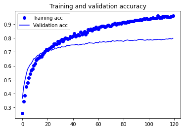
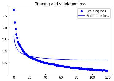
We’ll be covering two techniques to utilise our conv_base pretrained model. The first, demonstrated below, runs the convolutional base over our dataset, recording its output to Numpy arrays on disk. The resulting output, our image features, will be generated by calling the predict method of the conv_base model. This will serve as input to a standalone densely-connected classifier. While this first technique is computationally cheap to run, we will not be able to levarage data augmentation.
from pathlib import Path
def count_files(path, extension):
    directory = Path(path)
    return len(list(directory.glob('**/*.{extension}'.format(extension=extension))))
def extract_features(directory):
    sample_count = count_files(directory, 'jpg')

    features = np.zeros(shape=(sample_count, *conv_output_shape))
    labels = np.zeros(shape=(sample_count, len(classes)))

    datagen = ImageDataGenerator(rescale=1./255)

    generator = datagen.flow_from_directory(
        directory,
        classes=classes,
        target_size=train_generator.target_size,
        batch_size=batch_size,
        class_mode='categorical')

    i = 0
    for inputs_batch, labels_batch in generator:
        features_batch = conv_base.predict(inputs_batch)
        features[i * batch_size : (i + 1) * batch_size] = features_batch
        labels[i * batch_size : (i + 1) * batch_size] = labels_batch
        i += 1
        if i * batch_size >= sample_count:
            # Note that since generators yield data indefinitely in a loop,
            # we must `break` after every image has been seen once.
            break

    return features.reshape(-1, np.prod(conv_output_shape)), labels
    #return features, labels
x_train, y_train = extract_features(train_dir)
x_val, y_val = extract_features(validation_dir)
x_test, y_test = extract_features(test_dir)
Found 2590 images belonging to 5 classes.
Found 863 images belonging to 5 classes.
Found 864 images belonging to 5 classes.
Building our model
def build_model():
    model = models.Sequential()
    model.add(layers.Dense(512, activation='relu', input_dim=np.prod(conv_output_shape)))
    model.add(layers.Dropout(0.5))
    model.add(layers.Dense(len(classes), activation='softmax'))

    print(model.summary())

    model.compile(loss='categorical_crossentropy',
                  optimizer=optimizers.RMSprop(learning_rate=1.5e-6),
                  metrics =['categorical_accuracy'])

    return model
model = build_model()
Model: "sequential_2"
_________________________________________________________________
Layer (type)                 Output Shape              Param #
=================================================================
dense_4 (Dense)              (None, 512)               9437696
_________________________________________________________________
dropout_1 (Dropout)          (None, 512)               0
_________________________________________________________________
dense_5 (Dense)              (None, 5)                 2565
=================================================================
Total params: 9,440,261
Trainable params: 9,440,261
Non-trainable params: 0
_________________________________________________________________
None
def train_model(model, x_train, y_train, batch_size, epochs):
    history = model.fit(
        x_train,
        y_train,
        epochs=epochs,
        batch_size=batch_size,
        validation_data=(x_val, y_val)
    )

    plot_history(history)
train_model(model, x_train, y_train, batch_size, epochs=120)
Epoch 1/120
21/21 [==============================] - 1s 25ms/step - loss: 2.9395 - categorical_accuracy: 0.2490 - val_loss: 1.6137 - val_categorical_accuracy: 0.3662
Epoch 2/120
21/21 [==============================] - 0s 12ms/step - loss: 2.2237 - categorical_accuracy: 0.3449 - val_loss: 1.3728 - val_categorical_accuracy: 0.4484
Epoch 3/120
21/21 [==============================] - 0s 13ms/step - loss: 1.9830 - categorical_accuracy: 0.3764 - val_loss: 1.2408 - val_categorical_accuracy: 0.4959
Epoch 4/120
21/21 [==============================] - 0s 12ms/step - loss: 1.7783 - categorical_accuracy: 0.4306 - val_loss: 1.1490 - val_categorical_accuracy: 0.5365
Epoch 5/120
21/21 [==============================] - 0s 12ms/step - loss: 1.5726 - categorical_accuracy: 0.4829 - val_loss: 1.0828 - val_categorical_accuracy: 0.5736
Epoch 6/120
21/21 [==============================] - 0s 13ms/step - loss: 1.4134 - categorical_accuracy: 0.5195 - val_loss: 1.0380 - val_categorical_accuracy: 0.5898
Epoch 7/120
21/21 [==============================] - 0s 12ms/step - loss: 1.3547 - categorical_accuracy: 0.5381 - val_loss: 0.9956 - val_categorical_accuracy: 0.6072
Epoch 8/120
21/21 [==============================] - 0s 13ms/step - loss: 1.2626 - categorical_accuracy: 0.5754 - val_loss: 0.9650 - val_categorical_accuracy: 0.6165
Epoch 9/120
21/21 [==============================] - 0s 12ms/step - loss: 1.2131 - categorical_accuracy: 0.5718 - val_loss: 0.9386 - val_categorical_accuracy: 0.6327
Epoch 10/120
21/21 [==============================] - 0s 12ms/step - loss: 1.1475 - categorical_accuracy: 0.5981 - val_loss: 0.9156 - val_categorical_accuracy: 0.6512
...
Epoch 110/120
21/21 [==============================] - 0s 13ms/step - loss: 0.1864 - categorical_accuracy: 0.9497 - val_loss: 0.6135 - val_categorical_accuracy: 0.7879
Epoch 111/120
21/21 [==============================] - 0s 12ms/step - loss: 0.1909 - categorical_accuracy: 0.9471 - val_loss: 0.6133 - val_categorical_accuracy: 0.7868
Epoch 112/120
21/21 [==============================] - 0s 12ms/step - loss: 0.1855 - categorical_accuracy: 0.9505 - val_loss: 0.6178 - val_categorical_accuracy: 0.7903
Epoch 113/120
21/21 [==============================] - 0s 12ms/step - loss: 0.1775 - categorical_accuracy: 0.9506 - val_loss: 0.6148 - val_categorical_accuracy: 0.7891
Epoch 114/120
21/21 [==============================] - 0s 12ms/step - loss: 0.1768 - categorical_accuracy: 0.9540 - val_loss: 0.6143 - val_categorical_accuracy: 0.7914
Epoch 115/120
21/21 [==============================] - 0s 12ms/step - loss: 0.1796 - categorical_accuracy: 0.9501 - val_loss: 0.6151 - val_categorical_accuracy: 0.7926
Epoch 116/120
21/21 [==============================] - 0s 12ms/step - loss: 0.1719 - categorical_accuracy: 0.9539 - val_loss: 0.6150 - val_categorical_accuracy: 0.7914
Epoch 117/120
21/21 [==============================] - 0s 13ms/step - loss: 0.1827 - categorical_accuracy: 0.9476 - val_loss: 0.6120 - val_categorical_accuracy: 0.7949
Epoch 118/120
21/21 [==============================] - 0s 13ms/step - loss: 0.1575 - categorical_accuracy: 0.9548 - val_loss: 0.6133 - val_categorical_accuracy: 0.7949
Epoch 119/120
21/21 [==============================] - 0s 12ms/step - loss: 0.1748 - categorical_accuracy: 0.9575 - val_loss: 0.6134 - val_categorical_accuracy: 0.7926
Epoch 120/120
21/21 [==============================] - 0s 12ms/step - loss: 0.1608 - categorical_accuracy: 0.9589 - val_loss: 0.6127 - val_categorical_accuracy: 0.7984
y_pred = model.predict_classes(x_test)
print('-'*10 + 'Classification Report' + '-'*5)
print(classification_report(np.argmax(y_test, axis=1), y_pred, target_names=classes))
print('-'*10 + 'Confusion Matrix' + '-'*10)
plot_confusion_matrix(confusion_matrix(np.argmax(y_test, axis=1), y_pred))
----------Classification Report-----
              precision    recall  f1-score   support

       daisy       0.82      0.81      0.81       139
   dandelion       0.89      0.87      0.88       209
        rose       0.77      0.74      0.75       151
   sunflower       0.87      0.81      0.84       166
       tulip       0.75      0.85      0.80       199

    accuracy                           0.82       864
   macro avg       0.82      0.81      0.82       864
weighted avg       0.82      0.82      0.82       864

----------Confusion Matrix----------
Feature extraction with data augmentation
- Modify your program to include an image transformer. Train a new model.
- Apply your network to the test set and report the accuracy as well as the confusion matrix you obtained.
WARNING: “This technique is so expensive that you should only attempt it if you have access to a GPU–it’s absolutely intractable on CPU. If you can’t run your code on GPU, then the previous technique is the way to go” (F. Chollet, p.149).
Thankfully, Google provides us free access to a Tesla K80 GPU or equivalent on the Colab platform. To enable GPU hardware acceleration, go to Edit > Notebook settings and select GPU as our Hardware accelerator.
We can verify that our GPU is connected with the following script:
import tensorflow as tf
tf.test.gpu_device_name()
'/device:GPU:0'
If you see a device name after running the above, you’re good to go!
epochs = 20
batch_size = 128
target_size = (150, 150)
conv_base = InceptionV3(weights='imagenet',
                        include_top=False,
                        input_shape=(150, 150, 3))
Building our model
In this technique, we will be extending our model using the conv_base as a layer in our network. We can do so by adding Dense layers on top and running the whole thing end-to-end on the input data. This technique allows us to use data augmentation, because every input image is going through the convolutional base every time it is seen by the model. However, for this same reason, this technique is far more expensive than the first one.
Before we compile and train our model, we have to freeze the pretrained network weights. In other words, we want to prevent the conv_base weights from being updated during the training process. This is an important step since the use of randomly-initialised Dense layers would propagate very large weight updates through the network, effectively destroying the representations previously learned (Chollet, p.150).
# Freeze pretrained network weights
conv_base.trainable = False
def build_model(conv_base):
    model3 = models.Sequential()
    model3.add(conv_base)
    model3.add(layers.Flatten())
    model3.add(layers.Dropout(0.2))
    model3.add(layers.Dense(64, activation='relu'))
    model3.add(layers.Dense(len(classes), activation='softmax'))

    model3.compile(loss='categorical_crossentropy',
                      optimizer=optimizers.RMSprop(learning_rate=1e-4),
                      metrics =['categorical_accuracy'])

    return model3
model = build_model(conv_base)
def train_model(model, epochs=1):

    train_datagen = ImageDataGenerator(
        rescale=1./255,
        rotation_range=40,
        width_shift_range=0.2,
        height_shift_range=0.2,
        shear_range=0.2,
        zoom_range=0.2,
        horizontal_flip=True,
        fill_mode='nearest')

    test_datagen = ImageDataGenerator(rescale=1./255)

    train_generator = train_datagen.flow_from_directory(
        # This is the target directory
        train_dir,
        # All images will be resized to 150x150
        target_size=target_size,
        batch_size=batch_size,
        class_mode='categorical')

    # Note that validation data shouldn't be augmented
    validation_generator = test_datagen.flow_from_directory(
        validation_dir,
        target_size=(150, 150),
        batch_size=batch_size,
        class_mode='categorical'
    )

    history = model.fit_generator(
        train_generator,
        steps_per_epoch=np.ceil(train_generator.samples / train_generator.batch_size),
        epochs=epochs,
        validation_data=validation_generator,
        validation_steps=np.ceil(validation_generator.samples / validation_generator.batch_size))

    plot_history(history)
train_model(model, epochs=30)
Found 2590 images belonging to 5 classes.
Found 863 images belonging to 5 classes.


Epoch 1/30
21/21 [==============================] - 32s 1s/step - loss: 1.9633 - categorical_accuracy: 0.4219 - val_loss: 0.9103 - val_categorical_accuracy: 0.6419
Epoch 2/30
21/21 [==============================] - 19s 922ms/step - loss: 0.8563 - categorical_accuracy: 0.6613 - val_loss: 0.7963 - val_categorical_accuracy: 0.6860
Epoch 3/30
21/21 [==============================] - 19s 925ms/step - loss: 0.7653 - categorical_accuracy: 0.7012 - val_loss: 0.7185 - val_categorical_accuracy: 0.7358
Epoch 4/30
21/21 [==============================] - 20s 949ms/step - loss: 0.6763 - categorical_accuracy: 0.7325 - val_loss: 0.6431 - val_categorical_accuracy: 0.7555
Epoch 5/30
21/21 [==============================] - 20s 953ms/step - loss: 0.6222 - categorical_accuracy: 0.7737 - val_loss: 0.6396 - val_categorical_accuracy: 0.7717
Epoch 6/30
21/21 [==============================] - 20s 944ms/step - loss: 0.6140 - categorical_accuracy: 0.7770 - val_loss: 0.6381 - val_categorical_accuracy: 0.7555
Epoch 7/30
21/21 [==============================] - 19s 922ms/step - loss: 0.6045 - categorical_accuracy: 0.7803 - val_loss: 0.5965 - val_categorical_accuracy: 0.7961
Epoch 8/30
21/21 [==============================] - 19s 926ms/step - loss: 0.6140 - categorical_accuracy: 0.7696 - val_loss: 0.6222 - val_categorical_accuracy: 0.7856
Epoch 9/30
21/21 [==============================] - 20s 928ms/step - loss: 0.5334 - categorical_accuracy: 0.7951 - val_loss: 0.5765 - val_categorical_accuracy: 0.7926
Epoch 10/30
21/21 [==============================] - 19s 921ms/step - loss: 0.5232 - categorical_accuracy: 0.8119 - val_loss: 0.5962 - val_categorical_accuracy: 0.7879
...
Epoch 20/30
21/21 [==============================] - 19s 921ms/step - loss: 0.3916 - categorical_accuracy: 0.8543 - val_loss: 0.5594 - val_categorical_accuracy: 0.8053
Epoch 21/30
21/21 [==============================] - 19s 928ms/step - loss: 0.4193 - categorical_accuracy: 0.8464 - val_loss: 0.5475 - val_categorical_accuracy: 0.8065
Epoch 22/30
21/21 [==============================] - 20s 933ms/step - loss: 0.3727 - categorical_accuracy: 0.8638 - val_loss: 0.5457 - val_categorical_accuracy: 0.8192
Epoch 23/30
21/21 [==============================] - 20s 935ms/step - loss: 0.3791 - categorical_accuracy: 0.8545 - val_loss: 0.5680 - val_categorical_accuracy: 0.8053
Epoch 24/30
21/21 [==============================] - 19s 924ms/step - loss: 0.3906 - categorical_accuracy: 0.8630 - val_loss: 0.5972 - val_categorical_accuracy: 0.8065
Epoch 25/30
21/21 [==============================] - 19s 924ms/step - loss: 0.3976 - categorical_accuracy: 0.8516 - val_loss: 0.5696 - val_categorical_accuracy: 0.8053
Epoch 26/30
21/21 [==============================] - 20s 943ms/step - loss: 0.3617 - categorical_accuracy: 0.8621 - val_loss: 0.5650 - val_categorical_accuracy: 0.8053
Epoch 27/30
21/21 [==============================] - 20s 938ms/step - loss: 0.3871 - categorical_accuracy: 0.8551 - val_loss: 0.5768 - val_categorical_accuracy: 0.8088
Epoch 28/30
21/21 [==============================] - 20s 934ms/step - loss: 0.3260 - categorical_accuracy: 0.8821 - val_loss: 0.5836 - val_categorical_accuracy: 0.8111
Epoch 29/30
21/21 [==============================] - 20s 929ms/step - loss: 0.3462 - categorical_accuracy: 0.8788 - val_loss: 0.6000 - val_categorical_accuracy: 0.8134
Epoch 30/30
21/21 [==============================] - 20s 931ms/step - loss: 0.3354 - categorical_accuracy: 0.8708 - val_loss: 0.5690 - val_categorical_accuracy: 0.8134
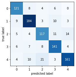
Evaluating model performance
def evaluate_model(model):
    test_generator = test_datagen.flow_from_directory(
        test_dir,
        shuffle=False,
        target_size=target_size,
        batch_size=batch_size,
        class_mode='categorical')

    y_prob = model.predict_generator(test_generator, np.ceil(test_generator.samples / test_generator.batch_size))
    y_pred = np.argmax(y_prob, axis=1)

    print('-'*10 + 'Classification Report' + '-'*5)
    print(classification_report(test_generator.classes, y_pred, target_names=classes))
    print('-'*10 + 'Confusion Matrix' + '-'*10)
    plot_confusion_matrix(confusion_matrix(test_generator.classes, y_pred))
evaluate_model(model)
Found 864 images belonging to 5 classes.


----------Classification Report-----
              precision    recall  f1-score   support

       daisy       0.83      0.87      0.85       139
   dandelion       0.86      0.88      0.87       209
        rose       0.76      0.77      0.77       151
   sunflower       0.82      0.85      0.84       166
       tulip       0.88      0.81      0.85       199

    accuracy                           0.84       864
   macro avg       0.83      0.84      0.84       864
weighted avg       0.84      0.84      0.84       864

----------Confusion Matrix----------
model.summary()
Model: "sequential_3"
_________________________________________________________________
Layer (type)                 Output Shape              Param #
=================================================================
module_wrapper (ModuleWrappe (None, 3, 3, 2048)        21802784
_________________________________________________________________
flatten_2 (Flatten)          (None, 18432)             0
_________________________________________________________________
dropout_2 (Dropout)          (None, 18432)             0
_________________________________________________________________
dense_6 (Dense)              (None, 64)                1179712
_________________________________________________________________
dense_7 (Dense)              (None, 5)                 325
=================================================================
Total params: 22,982,821
Trainable params: 1,180,037
Non-trainable params: 21,802,784
_________________________________________________________________
Fine-tuning
Fine-tuning refers to the unfreezing of a few layers in the conv_base frozen model base. We choose to unfreeze the layers which encode more specialised features. These layers in the InceptionV3 are at the top of the network.
Warning: Before we proceed, make sure that you have already trained your fully-connected classifier from above.
To further clarify, we will be re-purposing the InceptionV3 pre-trained model by fine-tuning the layers in the base. We already removed the convolutional base’s original classifier by setting include_top=False, which allowed us to use only the layers in the base which contained abstract representations of features useful for general image classification tasks. We then added our own fully-connected classifier to the network that allowed us to restrict the predictions to our specific problem domain (predicting the five classes of the flowers dataset). In order to preserve the InceptionV3’s learned weight values, we set conv_base.trainable = False. This step froze all the pre-trained model layers and kept their weight values the same during the training process. Now, we want to fine-tune our pre-trained model by setting some of the conv_base top layers to layer.trainable = True. We choose to unfreeze the higher layers whose specific features are said to be problem dependendent, as opposed to the lower layers whose general features are problem independent.
The figure below illustrates the two strategies we use in this notebook.
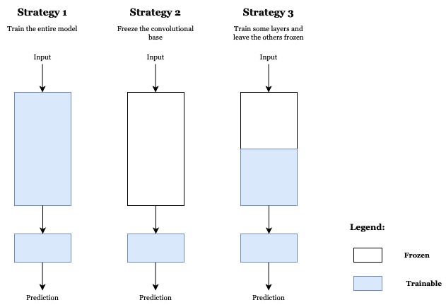 |
|---|
| Figure 1. Fine-tuning strategies. |
Strategy 2 was used previously to train only the fully-connected layers, while Strategy 3 will now be used to train both the fully-connected layers and some of the InceptionV3 top layers.
To help you choose which of the three transfer learning strategies is best for your specific dataset, you can refer to the following size-similarity perceptual map.
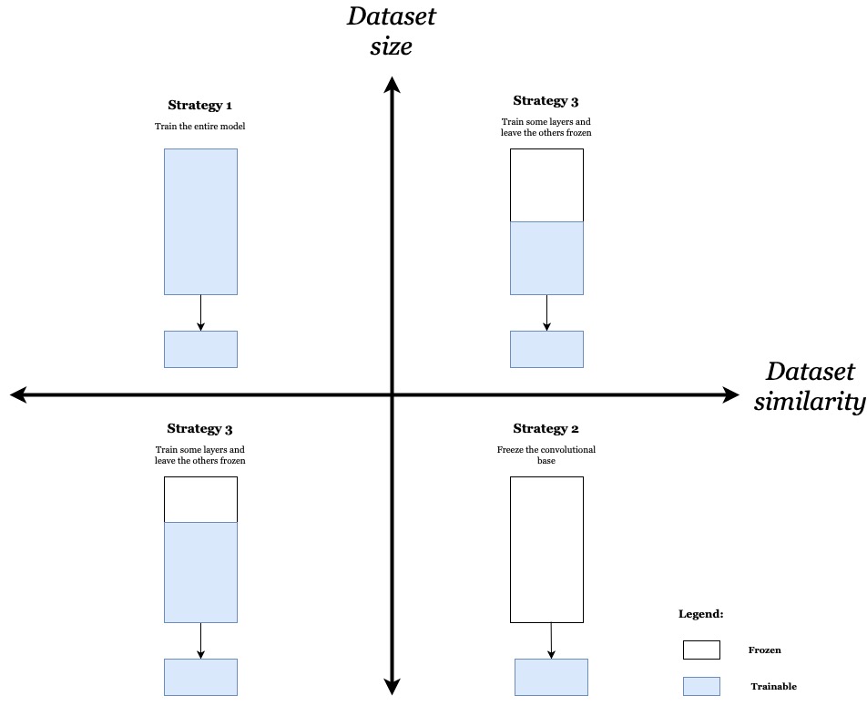 |
|---|
| Figure 2. Size-similarity perceptual map. |
Since we started off with a relatively small dataset, we chose Strategy 2 (Quadrant IV–small dataset, similar to pre-trained model dataset). We removed the original output layer from the InceptionV3 and ran the pre-trained model as a fixed feature extractor. The resulting features were used to train a new classifier, the fully-connected classifier we created in the previous model. In the model below, we will be assuming a balance between Quadrants I and III (small dataset, somewhat dissimilar to pre-trained model dataset).
import keras
print('Num layers in InceptionV3 base:', len(conv_base.layers))
Num layers in InceptionV3 base: 311
conv_base.trainable = True
### Fine-tuning
# set all layers trainable by default
for layer in conv_base.layers:
    layer.trainable = True
    if isinstance(layer, keras.layers.BatchNormalization):
        # we do aggressive exponential smoothing of batch norm
        # parameters to faster adjust to our new dataset
        layer.momentum = 0.9

# fix deep layers (fine-tuning only last 50 layers)
for layer in conv_base.layers[:-50]:
    # fix all but batch norm layers, because we neeed to update moving averages for a new dataset!
    if not isinstance(layer, keras.layers.BatchNormalization):
        layer.trainable = False
We will be using the RMSprop optimiser with a very low learning rate in order to limit the magnitude of the modifications made to the representations of the layers that we are fine-tuning. Updates that are too large might harm these representations (F. Chollet, p.178).
### Re-training model
model.compile(loss='categorical_crossentropy',
              optimizer=optimizers.RMSprop(learning_rate=1e-5),
              metrics =['categorical_accuracy'])

train_model(model, epochs=100)
Found 2590 images belonging to 5 classes.
Found 863 images belonging to 5 classes.


Epoch 1/100
21/21 [==============================] - 26s 983ms/step - loss: 0.5971 - categorical_accuracy: 0.8066 - val_loss: 0.5678 - val_categorical_accuracy: 0.8227
Epoch 2/100
21/21 [==============================] - 19s 927ms/step - loss: 0.5228 - categorical_accuracy: 0.8208 - val_loss: 0.5713 - val_categorical_accuracy: 0.8088
Epoch 3/100
21/21 [==============================] - 20s 932ms/step - loss: 0.4591 - categorical_accuracy: 0.8457 - val_loss: 0.5691 - val_categorical_accuracy: 0.8134
Epoch 4/100
21/21 [==============================] - 20s 932ms/step - loss: 0.4504 - categorical_accuracy: 0.8404 - val_loss: 0.5643 - val_categorical_accuracy: 0.8146
Epoch 5/100
21/21 [==============================] - 20s 935ms/step - loss: 0.4280 - categorical_accuracy: 0.8486 - val_loss: 0.5726 - val_categorical_accuracy: 0.8065
Epoch 6/100
21/21 [==============================] - 20s 931ms/step - loss: 0.3871 - categorical_accuracy: 0.8795 - val_loss: 0.5663 - val_categorical_accuracy: 0.8100
Epoch 7/100
21/21 [==============================] - 19s 928ms/step - loss: 0.3933 - categorical_accuracy: 0.8676 - val_loss: 0.5666 - val_categorical_accuracy: 0.8146
Epoch 8/100
21/21 [==============================] - 19s 928ms/step - loss: 0.3817 - categorical_accuracy: 0.8726 - val_loss: 0.5604 - val_categorical_accuracy: 0.8169
Epoch 9/100
21/21 [==============================] - 20s 941ms/step - loss: 0.3541 - categorical_accuracy: 0.8825 - val_loss: 0.5600 - val_categorical_accuracy: 0.8227
Epoch 10/100
21/21 [==============================] - 20s 930ms/step - loss: 0.3648 - categorical_accuracy: 0.8859 - val_loss: 0.5632 - val_categorical_accuracy: 0.8169
...
Epoch 90/100
21/21 [==============================] - 20s 932ms/step - loss: 0.1292 - categorical_accuracy: 0.9536 - val_loss: 0.5295 - val_categorical_accuracy: 0.8540
Epoch 91/100
21/21 [==============================] - 20s 936ms/step - loss: 0.1279 - categorical_accuracy: 0.9586 - val_loss: 0.5352 - val_categorical_accuracy: 0.8563
Epoch 92/100
21/21 [==============================] - 20s 931ms/step - loss: 0.1276 - categorical_accuracy: 0.9613 - val_loss: 0.5337 - val_categorical_accuracy: 0.8528
Epoch 93/100
21/21 [==============================] - 19s 926ms/step - loss: 0.1210 - categorical_accuracy: 0.9627 - val_loss: 0.5336 - val_categorical_accuracy: 0.8517
Epoch 94/100
21/21 [==============================] - 19s 927ms/step - loss: 0.1104 - categorical_accuracy: 0.9630 - val_loss: 0.5376 - val_categorical_accuracy: 0.8552
Epoch 95/100
21/21 [==============================] - 20s 939ms/step - loss: 0.1282 - categorical_accuracy: 0.9582 - val_loss: 0.5472 - val_categorical_accuracy: 0.8552
Epoch 96/100
21/21 [==============================] - 19s 927ms/step - loss: 0.1279 - categorical_accuracy: 0.9556 - val_loss: 0.5524 - val_categorical_accuracy: 0.8505
Epoch 97/100
21/21 [==============================] - 20s 929ms/step - loss: 0.1331 - categorical_accuracy: 0.9517 - val_loss: 0.5479 - val_categorical_accuracy: 0.8494
Epoch 98/100
21/21 [==============================] - 20s 934ms/step - loss: 0.1214 - categorical_accuracy: 0.9539 - val_loss: 0.5392 - val_categorical_accuracy: 0.8540
Epoch 99/100
21/21 [==============================] - 20s 929ms/step - loss: 0.1234 - categorical_accuracy: 0.9583 - val_loss: 0.5318 - val_categorical_accuracy: 0.8540
Epoch 100/100
21/21 [==============================] - 20s 936ms/step - loss: 0.1218 - categorical_accuracy: 0.9609 - val_loss: 0.5335 - val_categorical_accuracy: 0.8505
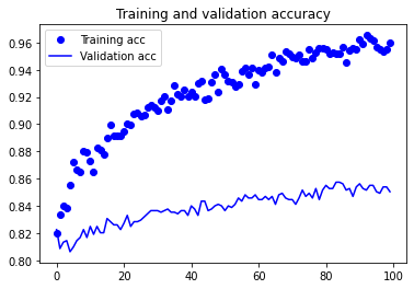
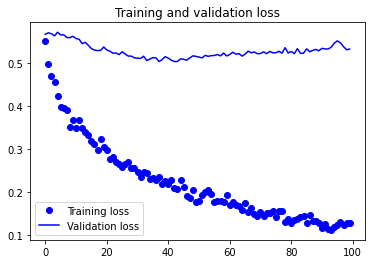
### Evaluating model performance
evaluate_model(model)
Found 864 images belonging to 5 classes.


----------Classification Report-----
              precision    recall  f1-score   support

       daisy       0.86      0.84      0.85       139
   dandelion       0.90      0.90      0.90       209
        rose       0.86      0.83      0.84       151
   sunflower       0.89      0.86      0.88       166
       tulip       0.84      0.90      0.87       199

    accuracy                           0.87       864
   macro avg       0.87      0.87      0.87       864
weighted avg       0.87      0.87      0.87       864

----------Confusion Matrix----------
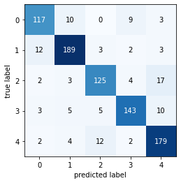
Great news–we were able to improve our model’s F1 score ca. 3% by fine-tuning our pre-trained convolutional base. Unfreezing some of the layers in the base let us successfully repurpose the pre-trained model weights to better fit our task. Let’s save our final model and call it a day! Thanks for sticking around this far.
### Saving final model
model.save('flowers_final.h5')
Credits
This assignment was prepared by Pierre Nugues, an extroadinary professor of Semantic Systems and Language Technology at Lunds Tekniska Högskola. More about him can be found here. Most of the inspiration for this notebook came from François Chollet, creator of Keras and author of Deep Learning with Python. His version of this task is found in notebooks 5.2-using-convnets-with-small-datasets.ipynb and 5.3-using-a-pretrained-convnet.ipynb. Another version can be found on the TensorFlow Guide blog here. Pedro Marcelino helped inspire Figures 1 and 2 in Fine-tuning, link to his article here. Also, special thanks to Alexander Maemev on Kaggle for the Flowers Recognition dataset used in this task, available publicly at the link here.
2019-11-22 00:00:00 -0800 - Written by Jonathan Logan Moran