NCC NBC GNBC scikit-learn digits MNIST classification machine-learning python ipynb Comparing the Performance of Various Classifiers on Handwritten Digits Datasets
In this post we will implement an NCC, a discrete (count-based) NBC, and a Gaussian NBC and run and compare them on different versions of the data set(s) in Section 2:
1. Classifiers
1.1. Scikit-learn Gaussian Naive Bayes Classifier
Make use of the provided Gaussian NB Classifier (sklearn.naive_bayes GaussianNB) for all data sets as a comparison.
from sklearn.naive_bayes import GaussianNB
class sklearnGNB:
    def fit(self, X_train, y_train):
        self.model = GaussianNB()
        self.model.fit(X_train, y_train)
        return self.model
    def predict(self, X_test):
        return self.model.predict(X_test)
1.2. Nearest Centroid Classifier
Implement your own Nearest Centroid Classifier (NCC): The NCC fit method should simply compute the mean values over the attribute values of the examples for each class. Prediction is then done by finding the argmin over the distances from the class centroids for each sample. This classifier should be run on all three variants of data sets, see below.
import numpy as np
class NCC:
    def fit(self, X_train, y_train):
        n_samples, n_features = X_train.shape
        self._classes = np.unique(y_train)
        n_classes = len(self._classes)
        self._centroids = np.zeros(shape=(n_classes, n_features))
        # Compute the per-class centroids (means)
        for cls in self._classes:
            idxs = np.where(y_train==cls)    # fetch all samples per label (class)
            # compute the mean value of each 16-bit image
            self._centroids[cls] = np.mean(X_train[idxs], axis=0)
        return self
    def predict(self, X_test):
        preds = np.zeros(shape=(len(X_test), n_classes))
        for i, x in enumerate(X_test):
            # compute dist to per-class centers
            preds[i] = [np.linalg.norm(x - centroid) for centroid in self._centroids]
        y_pred = np.argmin(preds, axis=1)
        return y_pred
1.3. Naive Bayes Classifier
Implement a Naive Bayesian Classifier (NBC) based on discrete (statistical) values (i.e., counts of examples falling into the different classes and attribute value groups) both for the priors and for the conditional probabilities. Run this on the two Scikit-learn digits data sets. It should also work with the (non-normalised) MNIST_Light set, but it will probably take a (very long) while and not give anything interesting really…
from itertools import product
class NBC:
    def fit(self, X_train, y_train, data="digits"):
        n_samples, n_rows, n_cols = np.shape(X_train)
        self._classes, self.class_counts = np.unique(y_train, return_counts=True)
        # 1. Compute class priors: digit frequency
        class_priors = self.class_counts / np.sum(self.class_counts)
        # 2. Compute attribute likelihoods
        likelihoods = {}
        pixel_values = np.unique(X_train.flatten())
        for cls in self._classes:
            # store class atrribute frequencies
            cls_pixels = {}
            # get all samples in current class
            idxs = np.where(y_train == cls)
            # iterate over each image and its coordinates
            for k, (i,j) in enumerate(product(range(n_rows), range(n_cols))):
                # store attribute value counts (number of occurences)
                cls_pixel_counts = np.zeros(shape=len(pixel_values))
                # get attribute value at pixel location and count num occurences in current class
                loc, num_occurences = np.unique(X_train[idxs][:,i,j], return_counts=True)
                # store attribute value class occurences for every pixel location in image
                cls_pixel_counts[loc.astype(np.int8)] = num_occurences
                # compute attribute value class frequencies
                if data is "digits":
                    # with Laplace smoothing
                    freq = (cls_pixel_counts + 1) / np.sum(cls_pixel_counts + 1)
                else:
                    freq = cls_pixel_counts / np.sum(cls_pixel_counts)
                cls_pixels.update({k:freq})
            likelihoods[cls] = cls_pixels
        self._likelihoods = likelihoods
        self._class_priors = class_priors
        self._data = data
        return self
    def predict(self, X_test):
        n_samples, n_rows, n_cols = np.shape(X_test)
        y_pred = np.zeros(shape=len(X_test))
        for n, x in enumerate(X_test):
            posterior = np.zeros(len(self._classes))
            for cls in self._classes:
                prob = self._class_priors[cls]
                for k, (i,j) in enumerate(product(range(n_rows), range(n_cols))):
                    # 3. Compute conditional probability of seeing pixel value at location (i,j) in image k
                    prob *= self._likelihoods[cls][k][int(x[i,j])]
                posterior[cls] = self._class_priors[cls] * prob
            y_pred[n] = np.argmax(posterior)
        return y_pred
1.4. Gaussian Naive Bayes Classifier
import math
class GNBC:
    def log_likelihood(self, x, mu, sigma):
        epsilon = 1e-4
        coeff = 1.0 / np.sqrt(2.0 * math.pi * sigma + epsilon)
        exponent = math.exp(-1.0 * (x - mu)**2 / (2.0 * sigma + epsilon))
        return np.log(coeff * exponent)
    def fit(self, X_train, y_train):
        self._classes, self.class_counts = np.unique(y_train, return_counts=True)
        # 1. Compute class priors
        self._class_priors = self.class_counts / np.sum(self.class_counts)
        # 2. Compute Gaussian distribution parameters
        means = {}
        vars = {}
        for cls in self._classes:
            # get all samples in class
            idxs = np.where(y_train == cls)
            # compute class mean
            cls_mean = np.mean(X_train[idxs], axis=0)
            means.update({cls:cls_mean})
            # compute class variance
            cls_var = np.var(X_train[idxs], axis=0)
            vars.update({cls:cls_var})
        self._means = means
        self._vars = vars
    def predict(self, X_test):
        y_pred = np.zeros(len(X_test))
        log_likelihood = np.vectorize(self.log_likelihood)
        for i, x in enumerate(X_test):
            probs = np.zeros(len(self._classes))
            for cls in self._classes:
                # P(Y): class prior (frequency in training set)
                prior = self._class_priors[cls]
                # P(X|Y): probability of X given class distribution Y
                prob = log_likelihood(x, self._means[cls], self._vars[cls])
                # P(Y|X) = P(Y)*P(X|Y)
                posterior = prior * np.sum(prob)
                probs[cls] = posterior
            y_pred[i] = np.argmax(probs)
        return y_pred
2. Datasets
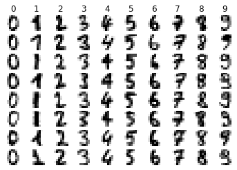
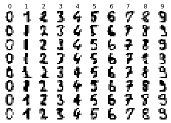
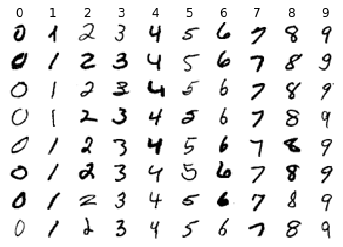
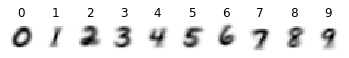
2.1. Scikit-learn Digits
Recall that the digits dataset consists of 1797 samples. Each sample is an 8x8 image of a single handwritten digit from 0 to 9. Each sample therefore has 64 features, where each of the 64 features is a brightness value of a pixel in the image.
from sklearn.datasets import load_digits
digits = load_digits()
# Classes in dataset
classes = np.unique(digits.target)
n_classes = len(classes)
import matplotlib.pyplot as plt
def visualize_random(images, labels, examples_per_class):
    """
    Display random sample of images per class
    """
    number_of_classes = len(np.unique(labels))

    for cls in range(number_of_classes):
        idxs = np.where(labels == cls)[0]
        idxs = np.random.choice(idxs, examples_per_class, replace=False)
        for i, idx in enumerate(idxs):
            plt.subplot(examples_per_class, number_of_classes, i * number_of_classes + cls + 1)
            plt.imshow(images[idx].astype('uint8'), cmap=plt.cm.gray_r, interpolation='nearest')
            plt.axis('off')
            if i == 0:
                plt.title(str(cls))
    plt.show()
visualize_random(digits.images, digits.target, 8)
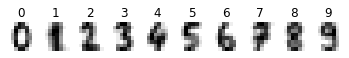
def mean_image(images, labels, dim):
    """
    Display mean image of each class
    """
    # Assume 10 classes, dimxdim image data
    cls_means = np.zeros(shape=(10,dim,dim))
    for cls in range(n_classes):
        idxs = np.where(labels == cls)[0]
        cls_means[cls] = np.mean(images[idxs], axis=0)
        plt.subplot(1, n_classes, cls + 1)
        plt.axis('off')
        plt.imshow(cls_means[cls].astype('uint8'), cmap=plt.cm.gray_r, interpolation='nearest')
        plt.title(str(cls))
    plt.show()
mean_image(digits.images, digits.target, dim=8)
from sklearn.model_selection import train_test_split
X_train, X_test, y_train, y_test = train_test_split(digits.images, digits.target, test_size=0.3)
# Normalise image data
X_train = X_train / 16.0
X_test = X_test / 16.0
2.1.1. Scikit-learn Gaussian Naive Bayes Classifier
# Reshape data to 2D
X_train = X_train.reshape((len(X_train), -1))
X_test = X_test.reshape((len(X_test), -1))
sklearnGNB = sklearnGNB()
sklearnGNB.fit(X_train, y_train)
GaussianNB(priors=None, var_smoothing=1e-09)
y_pred = sklearnGNB.predict(X_test)
from sklearn import metrics
from mlxtend.plotting import plot_confusion_matrix
print('Scikit-learn Guassian Naive Bayes Classifier on digits dataset... \n')
print('-'*10 + 'Classification Report' + '-'*5)
print(metrics.classification_report(y_test, y_pred))
print('-'*10 + 'Confusion Matrix' + '-'*10)
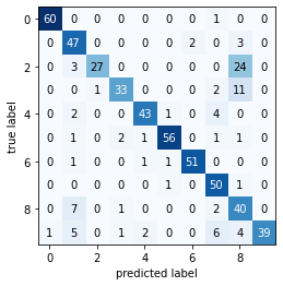
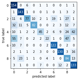
plot_confusion_matrix(metrics.confusion_matrix(y_test, y_pred))
Scikit-learn Guassian Naive Bayes Classifier on digits dataset...

----------Classification Report-----
              precision    recall  f1-score   support

           0       0.98      0.98      0.98        61
           1       0.71      0.90      0.80        52
           2       0.96      0.50      0.66        54
           3       0.89      0.70      0.79        47
           4       0.91      0.86      0.89        50
           5       0.95      0.90      0.93        62
           6       0.96      0.94      0.95        54
           7       0.76      0.96      0.85        52
           8       0.48      0.80      0.60        50
           9       1.00      0.67      0.80        58

    accuracy                           0.83       540
   macro avg       0.86      0.82      0.82       540
weighted avg       0.87      0.83      0.83       540

----------Confusion Matrix----------
2.1.2. Nearest Centroid Classifier
ncc = NCC()
ncc.fit(X_train, y_train)
y_pred = ncc.predict(X_test)
print('Nearest Centroid Classifier on digits dataset... \n')
print('-'*10 + 'Classification Report' + '-'*5)
print(metrics.classification_report(y_test, y_pred))
print('-'*10 + 'Confusion Matrix' + '-'*10)
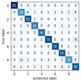
plot_confusion_matrix(metrics.confusion_matrix(y_test, y_pred))
Nearest Centroid Classifier on digits dataset...

----------Classification Report-----
              precision    recall  f1-score   support

           0       0.98      1.00      0.99        61
           1       0.78      0.73      0.75        52
           2       0.91      0.94      0.93        54
           3       0.93      0.89      0.91        47
           4       0.96      0.92      0.94        50
           5       0.93      0.89      0.91        62
           6       0.96      0.96      0.96        54
           7       0.86      0.98      0.92        52
           8       0.84      0.72      0.77        50
           9       0.77      0.86      0.81        58

    accuracy                           0.89       540
   macro avg       0.89      0.89      0.89       540
weighted avg       0.89      0.89      0.89       540

----------Confusion Matrix----------
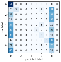
2.1.3. Naive Bayes Classifier
n_samples, n_pixels = X_train.shape
dim = int(np.sqrt(n_pixels))
# Reshape data to 3D
X_train_nbc = X_train.reshape((len(X_train), dim, dim))
X_test_nbc = X_test.reshape((len(X_test), dim, dim))
X_train_nbc.shape
(1257, 8, 8)
nbc = NBC()
nbc.fit(X_train_nbc, y_train)
y_pred = nbc.predict(X_test_nbc)
print('Naive Bayes Classifier on digits dataset... \n')
print('-'*10 + 'Classification Report' + '-'*5)
print(metrics.classification_report(y_test, y_pred))
print('-'*10 + 'Confusion Matrix' + '-'*10)
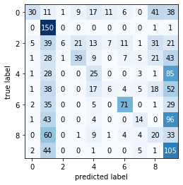
plot_confusion_matrix(metrics.confusion_matrix(y_test, y_pred))
Naive Bayes Classifier on digits dataset...

----------Classification Report-----
              precision    recall  f1-score   support

           0       0.22      1.00      0.36        61
           1       1.00      0.17      0.30        52
           2       0.00      0.00      0.00        54
           3       0.00      0.00      0.00        47
           4       0.00      0.00      0.00        50
           5       1.00      0.05      0.09        62
           6       0.43      0.11      0.18        54
           7       0.82      0.17      0.29        52
           8       0.12      0.56      0.20        50
           9       0.00      0.00      0.00        58

    accuracy                           0.21       540
   macro avg       0.36      0.21      0.14       540
weighted avg       0.37      0.21      0.14       540

----------Confusion Matrix----------
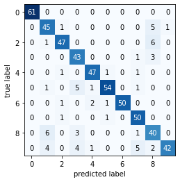
2.1.4. Gaussian Naive Bayes Classifier
gnbc = GNBC()
gnbc.fit(X_train, y_train)
y_pred = gnbc.predict(X_test)
print('Gaussian Naive Bayes Classifier on digits dataset... \n')
print('-'*10 + 'Classification Report' + '-'*5)
print(metrics.classification_report(y_test, y_pred))
print('-'*10 + 'Confusion Matrix' + '-'*10)
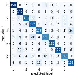
plot_confusion_matrix(metrics.confusion_matrix(y_test, y_pred))
Gaussian Naive Bayes Classifier on digits dataset...

----------Classification Report-----
              precision    recall  f1-score   support

           0       1.00      1.00      1.00        61
           1       0.79      0.87      0.83        52
           2       0.92      0.87      0.90        54
           3       0.78      0.91      0.84        47
           4       0.92      0.94      0.93        50
           5       0.95      0.87      0.91        62
           6       1.00      0.93      0.96        54
           7       0.85      0.96      0.90        52
           8       0.71      0.80      0.75        50
           9       0.98      0.72      0.83        58

    accuracy                           0.89       540
   macro avg       0.89      0.89      0.89       540
weighted avg       0.90      0.89      0.89       540

----------Confusion Matrix----------
2.2. Scikit-learn Digits Summarised
Reduce the digits data set to only contain three values for the attributes, e.g., 0 for dark, 1 for grey and 2 for light, with dark, grey and light. Split again into 70% training and 30% test data.
Bins:
- Light:
0-4 - Grey:
5-10 - Dark:
11-16
bin_bounds = [4, 10]
digits_data_summarised = np.digitize(digits.images, bins=bin_bounds, right=True)
digits_target_summarised = digits.target
# Display random sample of images per class
n_samples = 8
n_classes = 10
for cls in range(n_classes):
    idxs = np.where(digits_target_summarised == cls)[0]
    idxs = np.random.choice(idxs, n_samples, replace=False)
    for i, idx in enumerate(idxs):
        plt.subplot(n_samples, n_classes, i * n_classes + cls + 1)
        plt.axis('off')
        plt.imshow(digits_data_summarised[idx].reshape((8,8)).astype('uint8'), cmap=plt.cm.gray_r, interpolation='nearest')
        if i == 0:
            plt.title(str(cls))
plt.show()
X_train, X_test, y_train, y_test = train_test_split(digits_data_summarised, digits_target_summarised, test_size=0.3)
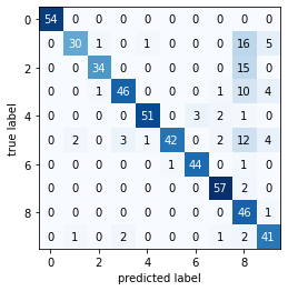
2.2.1. Scikit-learn Gaussian Naive Bayes Classifier
# Reshape data to 2D
X_train = X_train.reshape((len(X_train), -1))
X_test = X_test.reshape((len(X_test), -1))
sklearnGNB.fit(X_train, y_train)
GaussianNB(priors=None, var_smoothing=1e-09)
y_pred = sklearnGNB.predict(X_test)
print('Scikit-learn Gaussian Naive Bayes Classifier on digits summarised dataset... \n')
print('-'*10 + 'Classification Report' + '-'*5)
print(metrics.classification_report(y_test, y_pred))
print('-'*10 + 'Confusion Matrix' + '-'*10)
plot_confusion_matrix(metrics.confusion_matrix(y_test, y_pred))
Scikit-learn Gaussian Naive Bayes Classifier on digits summarised dataset...

----------Classification Report-----
              precision    recall  f1-score   support

           0       1.00      1.00      1.00        54
           1       0.91      0.57      0.70        53
           2       0.94      0.69      0.80        49
           3       0.90      0.74      0.81        62
           4       0.96      0.89      0.93        57
           5       0.98      0.64      0.77        66
           6       0.94      0.96      0.95        46
           7       0.90      0.97      0.93        59
           8       0.44      0.98      0.61        47
           9       0.75      0.87      0.80        47

    accuracy                           0.82       540
   macro avg       0.87      0.83      0.83       540
weighted avg       0.88      0.82      0.83       540

----------Confusion Matrix----------
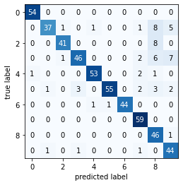
2.2.2. Nearest Centroid Classifier
ncc.fit(X_train, y_train)
y_pred = ncc.predict(X_test)
print('Nearest Centroid Classifier on digits summarised data... \n')
print('-'*10 + 'Classification Report' + '-'*5)
print(metrics.classification_report(y_test, y_pred))
print('-'*10 + 'Confusion Matrix' + '-'*10)
plot_confusion_matrix(metrics.confusion_matrix(y_test, y_pred))
Nearest Centroid Classifier on digits summarised data...

----------Classification Report-----
              precision    recall  f1-score   support

           0       0.98      1.00      0.99        54
           1       0.86      0.72      0.78        53
           2       0.91      0.86      0.88        49
           3       0.93      0.81      0.86        62
           4       1.00      0.98      0.99        57
           5       0.98      0.91      0.94        66
           6       0.96      0.98      0.97        46
           7       0.95      1.00      0.98        59
           8       0.83      0.85      0.84        47
           9       0.67      0.96      0.79        47

    accuracy                           0.91       540
   macro avg       0.91      0.91      0.90       540
weighted avg       0.91      0.91      0.91       540

----------Confusion Matrix----------
2.2.3. Naive Bayes Classifier
n_samples, n_pixels = X_train.shape
dim = int(np.sqrt(n_pixels))
# Reshape data to 3D
X_train_nbc = X_train.reshape((len(X_train), dim, dim))
X_test_nbc = X_test.reshape((len(X_test), dim, dim))
nbc.fit(X_train_nbc, y_train)
y_pred = nbc.predict(X_test_nbc)
print('Naive Bayes Classifier on digits summarised data... \n')
print('-'*10 + 'Classification Report' + '-'*5)
print(metrics.classification_report(y_test, y_pred))
print('-'*10 + 'Confusion Matrix' + '-'*10)
plot_confusion_matrix(metrics.confusion_matrix(y_test, y_pred))
Naive Bayes Classifier on digits summarised data...

----------Classification Report-----
              precision    recall  f1-score   support

           0       0.98      1.00      0.99        54
           1       0.87      0.75      0.81        53
           2       0.88      0.88      0.88        49
           3       0.96      0.79      0.87        62
           4       0.98      0.96      0.97        57
           5       1.00      0.91      0.95        66
           6       0.98      0.98      0.98        46
           7       0.94      1.00      0.97        59
           8       0.84      0.87      0.85        47
           9       0.71      0.98      0.82        47

    accuracy                           0.91       540
   macro avg       0.91      0.91      0.91       540
weighted avg       0.92      0.91      0.91       540

----------Confusion Matrix----------

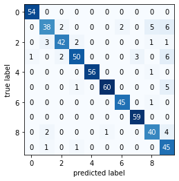
2.2.4. Gaussian Naive Bayes Classifier
gnbc.fit(X_train, y_train)
y_pred = gnbc.predict(X_test)
print('Gaussian Naive Bayes Classifier on digits summarised dataset... \n')
print('-'*10 + 'Classification Report' + '-'*5)
print(metrics.classification_report(y_test, y_pred))
print('-'*10 + 'Confusion Matrix' + '-'*10)
plot_confusion_matrix(metrics.confusion_matrix(y_test, y_pred))
Gaussian Naive Bayes Classifier on digits summarised dataset...

----------Classification Report-----
              precision    recall  f1-score   support

           0       0.98      1.00      0.99        54
           1       0.95      0.70      0.80        53
           2       0.95      0.84      0.89        49
           3       0.92      0.74      0.82        62
           4       0.96      0.93      0.95        57
           5       0.98      0.83      0.90        66
           6       1.00      0.96      0.98        46
           7       0.88      1.00      0.94        59
           8       0.64      0.98      0.77        47
           9       0.75      0.94      0.83        47

    accuracy                           0.89       540
   macro avg       0.90      0.89      0.89       540
weighted avg       0.91      0.89      0.89       540

----------Confusion Matrix----------
2.3. MNIST_Light
# ---------------------------------------------------------------- #
# This code is mainly from the EDAN95 fall term lab session No 6,
# provided by Volker Krueger
# ---------------------------------------------------------------- #
from PIL import Image
import glob

dir = 'src/MNIST_Light/*/*.png'

filelist = sorted(glob.glob(dir))
x = np.array([np.array(Image.open(fname)) for fname in filelist])

samples_per_class = 500
number_of_classes = 10

y = np.zeros(number_of_classes * samples_per_class, dtype=int)
for cls in range(1, number_of_classes):
    y[(cls*500):(cls+1)*500] = cls

train_features, test_features, train_labels, test_labels = train_test_split(x, y, test_size=0.3, random_state=42)
train_normalised = train_features.reshape(3500, 400) / 255.0
test_normalised = test_features.reshape(1500, 400) / 255.0
train_features.shape
(3500, 20, 20)
visualize_random(train_features, train_labels, examples_per_class=8)
mean_image(train_features, train_labels, dim=20)
2.3.1. Scikit-learn Gaussian Naive Bayes Classifier
sklearnGNB.fit(train_normalised, train_labels)
GaussianNB(priors=None, var_smoothing=1e-09)
y_pred = sklearnGNB.predict(test_normalised)
print('Scikit-learn Gaussian Naive Bayes Classifier on MNIST_Light data... \n')
print('-'*10 + 'Classification Report' + '-'*5)
print(metrics.classification_report(test_labels, y_pred))
print('-'*10 + 'Confusion Matrix' + '-'*10)
plot_confusion_matrix(metrics.confusion_matrix(test_labels, y_pred))
Scikit-learn Gaussian Naive Bayes Classifier on MNIST_Light data...

----------Classification Report-----
              precision    recall  f1-score   support

           0       0.54      0.94      0.69       164
           1       0.71      0.94      0.81       152
           2       0.83      0.50      0.62       155
           3       0.83      0.53      0.65       154
           4       0.75      0.31      0.44       143
           5       0.67      0.16      0.25       141
           6       0.81      0.85      0.83       143
           7       0.83      0.82      0.83       158
           8       0.41      0.64      0.50       132
           9       0.60      0.84      0.70       158

    accuracy                           0.66      1500
   macro avg       0.70      0.65      0.63      1500
weighted avg       0.70      0.66      0.64      1500

----------Confusion Matrix----------
2.3.2. Nearest Centroid Classifier
ncc.fit(train_normalised, train_labels)
y_pred = ncc.predict(test_normalised)
print('Nearest Centroid Classifier on MNIST_Light data... \n')
print('-'*10 + 'Classification Report' + '-'*5)
print(metrics.classification_report(test_labels, y_pred))
print('-'*10 + 'Confusion Matrix' + '-'*10)
plot_confusion_matrix(metrics.confusion_matrix(test_labels, y_pred))
Nearest Centroid Classifier on MNIST_Light data...

----------Classification Report-----
              precision    recall  f1-score   support

           0       0.91      0.91      0.91       164
           1       0.71      0.97      0.82       152
           2       0.84      0.73      0.78       155
           3       0.74      0.76      0.75       154
           4       0.75      0.76      0.75       143
           5       0.72      0.69      0.70       141
           6       0.90      0.86      0.88       143
           7       0.95      0.80      0.87       158
           8       0.79      0.72      0.75       132
           9       0.76      0.80      0.78       158

    accuracy                           0.80      1500
   macro avg       0.81      0.80      0.80      1500
weighted avg       0.81      0.80      0.80      1500

----------Confusion Matrix----------
2.3.3. Naive Bayes Classifier
n_samples, n_pixels = train_normalised.shape
dim = int(np.sqrt(n_pixels))
# Reshape data to 3D
train_normalised_nbc = train_normalised.reshape((len(train_normalised), dim, dim))
test_normalised_nbc = test_normalised.reshape((len(test_normalised), dim, dim))
nbc.fit(train_normalised_nbc, train_labels, data="MNIST_Light")
y_pred = nbc.predict(test_normalised_nbc)
print('Naive Bayes Classifier on MNIST_Light data... \n')
print('-'*10 + 'Classification Report' + '-'*5)
print(metrics.classification_report(test_labels, y_pred))
print('-'*10 + 'Confusion Matrix' + '-'*10)
plot_confusion_matrix(metrics.confusion_matrix(test_labels, y_pred))
Naive Bayes Classifier on MNIST_Light data...

----------Classification Report-----
              precision    recall  f1-score   support

           0       0.70      0.18      0.29       164
           1       0.32      0.99      0.48       152
           2       0.75      0.04      0.07       155
           3       0.56      0.25      0.35       154
           4       0.25      0.17      0.21       143
           5       0.24      0.04      0.07       141
           6       0.69      0.50      0.58       143
           7       0.38      0.09      0.14       158
           8       0.15      0.15      0.15       132
           9       0.21      0.66      0.32       158

    accuracy                           0.31      1500
   macro avg       0.42      0.31      0.27      1500
weighted avg       0.43      0.31      0.27      1500

----------Confusion Matrix----------
Credits
From the EDAN95 - Applied Machine Learning course given at Lunds Tekniska Högskola (LTH) | HT19. This assignment was prepared by V. Krueger, link here.
2019-12-06 00:00:00 -0800 - Written by Jonathan Logan Moran